Mathematica 中的插值

Question

请考虑以下分布：

rs={{400, 0.00929}, {410, 0.0348}, {420, 0.0966}, {430, 0.2}, {440, 0.328}, {450, 0.455}, 
    {460, 0.567}, {470, 0.676}, {480, 0.793}, {490, 0.904}, {500, 0.982}, {510, 0.997}, 
    {520,0.935}, {530, 0.811}, {540, 0.65}, {550, 0.481}, {560, 0.329}, {570,0.208}, 
    {580, 0.121}, {590, 0.0655}, {600, 0.0332}, {610, 0.0159}, {620, 0.00737}, 
    {630, 0.00334}, {640, 0.0015}, {650,0.000677}, {660, 0.000313}, {670, 0.000148}, 
    {680, 0.0000715}, {690,0.0000353}, {700, 0.0000178}}

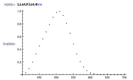
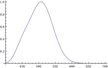
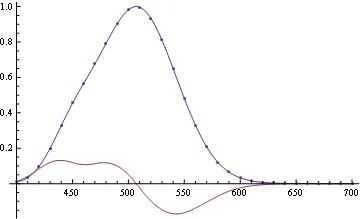
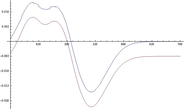
我该如何插值这个分布以获得 X 轴上任意位置的数值？

- 500

Answer 1

只需使用标准的插值函数：

rsInterpolation = Interpolation@rs;
Plot[rsInterpolation@x, {x, 400, 700}]

如果你想要适配于特定类别的函数（例如正态分布），请使用FindFit。

- Mechanical snail

---

请注意，Interpolation[]作为外推显然无法按预期工作。尝试使用Plot[Interpolation[rs]@x, {x, 1, 1000}]来查看。这不是本答案的缺陷！ - Dr. belisarius

@belisarius 哈哈，你的图表太可怕了。这是我使用它的方式，似乎可以工作：rsi = Interpolation[Transpose@{Range[400, 700, 10], Flatten@rodSensitivity}] rsi /@ Range[#,#+30,1] & /@ {440, 490, 540} - 500

我认为在这里不需要符合正态分布。这看起来像是人眼的敏感曲线（x轴表示波长，单位是纳米）。 - Sjoerd C. de Vries

@LeonidShifrin 嗯，我相信递归的隐灵正在工作。评论：删除此评论：删除这个... - Daniel Lichtblau

FixedPoint [@ Daniel's Comment [#]&，x] - Dr. belisarius

Answer 2

如果您需要美观的衍生品，可以这样做：

interp = Interpolation[rs, InterpolationOrder -> 3, Method -> "Spline"]
Show[Plot[{interp[x], 10 interp'[x]}, {x, Min[First /@ rs], Max[First /@ rs]},
          PlotRange -> Full],
     ListPlot@rs]

当你使用"样条插值"方法时，观察导数行为的差异：

interp  = Interpolation[rs, InterpolationOrder -> 3, Method -> "Spline"]
interp1 = Interpolation[rs, InterpolationOrder -> 3]
Show[Plot[{interp1'[x], interp'[x] - .005}, 
          {x, Min[First /@ rs], Max[First /@ rs]}, PlotRange -> Full]]

- Dr. belisarius

---

@yoda 我知道，但是我更喜欢明确指定。以防未来的版本更改了这一点 :) - Dr. belisarius

恭喜您获得金色Mathematica徽章！##派对喇叭## - Mr.Wizard

Answer 3

如果这是一个分布，我认为你应该使用 SmoothKernelDistribution。

- carlosayam