如何获取信号的高低包络

Question

我有一些嘈杂的数据，正在尝试制作高低包络线到信号。这有点像MATLAB中“提取峰值包络”的此示例。

Python中是否有类似的函数能够实现呢？我的整个项目都是用Python编写的，最坏的情况是我可以提取numpy数组并将其放入MATLAB中使用该示例。但我更喜欢matplotlib的外观... 真的很烦做所有的MATLAB和Python之间的I/O...

- user5224720

---

一个快速的谷歌搜索给我展示了这个链接：http://www.mathworks.com/matlabcentral/fileexchange/37545-envelope-detction-for-signal-analysis/content/envelope.m - DilithiumMatrix

还有这些：http://dsp.stackexchange.com/a/3464，https://dev59.com/NYzda4cB1Zd3GeqPhhFJ，http://scipy.github.io/devdocs/generated/scipy.signal.hilbert.html - DilithiumMatrix

Answer 1

第一次尝试是利用scipy Hilbert变换来确定振幅包络，但在许多情况下这并没有像预期的那样工作，主要原因是，引用自这个数字信号处理答案：

Hilbert包络，也称为能量-时间曲线（ETC），仅适用于窄带波动。生成一个解析信号，然后取绝对值，这是一种线性操作，因此它平等地处理信号的所有频率。如果您给它一个纯正弦波，它确实会返回直线。然而，当你给它白噪声时，你可能会得到噪声。

从那时起，由于其他答案使用了三次样条插值，往往变得笨重、不稳定（虚假振荡）和耗时，特别是对于非常长和嘈杂的数据数组，我将在这里提供一个简单和高效的numpy版本，似乎工作得非常好：

import numpy as np
from matplotlib import pyplot as plt

def hl_envelopes_idx(s, dmin=1, dmax=1, split=False):
    """
    Input :
    s: 1d-array, data signal from which to extract high and low envelopes
    dmin, dmax: int, optional, size of chunks, use this if the size of the input signal is too big
    split: bool, optional, if True, split the signal in half along its mean, might help to generate the envelope in some cases
    Output :
    lmin,lmax : high/low envelope idx of input signal s
    """

    # locals min      
    lmin = (np.diff(np.sign(np.diff(s))) > 0).nonzero()[0] + 1 
    # locals max
    lmax = (np.diff(np.sign(np.diff(s))) < 0).nonzero()[0] + 1 
    
    if split:
        # s_mid is zero if s centered around x-axis or more generally mean of signal
        s_mid = np.mean(s) 
        # pre-sorting of locals min based on relative position with respect to s_mid 
        lmin = lmin[s[lmin]<s_mid]
        # pre-sorting of local max based on relative position with respect to s_mid 
        lmax = lmax[s[lmax]>s_mid]

    # global min of dmin-chunks of locals min 
    lmin = lmin[[i+np.argmin(s[lmin[i:i+dmin]]) for i in range(0,len(lmin),dmin)]]
    # global max of dmax-chunks of locals max 
    lmax = lmax[[i+np.argmax(s[lmax[i:i+dmax]]) for i in range(0,len(lmax),dmax)]]
    
    return lmin,lmax

例子1：准周期振动

t = np.linspace(0,8*np.pi,5000)
s = 0.8*np.cos(t)**3 + 0.5*np.sin(np.exp(1)*t)
lmin, lmax = hl_envelopes_idx(s)

# plot
plt.plot(t,s,label='signal')
plt.plot(t[lmin], s[lmin], 'r', label='low')
plt.plot(t[lmax], s[lmax], 'g', label='high')

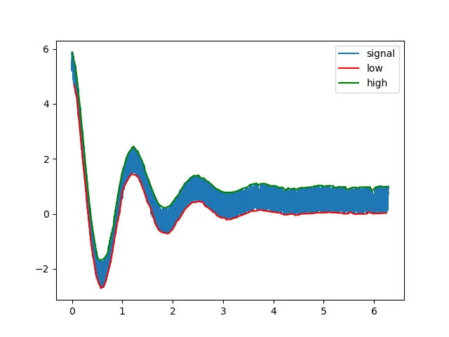
示例2：嘈杂衰减信号

t = np.linspace(0,2*np.pi,5000)
s = 5*np.cos(5*t)*np.exp(-t) + np.random.rand(len(t))

lmin, lmax = hl_envelopes_idx(s,dmin=15,dmax=15)

# plot
plt.plot(t,s,label='signal')
plt.plot(t[lmin], s[lmin], 'r', label='low')
plt.plot(t[lmax], s[lmax], 'g', label='high')

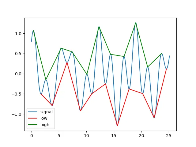
示例3：非对称调制啁啾信号

一个更加复杂的信号，包含18867925个样本（此处未包含）：

- Yacola

---

这个回答的信用度不够高，但这是目前为止最简单的方法。 - Alfonso Santiago

Hilbert方法的局限性有一个好的引言。寻找峰值和谷值的方法非常优雅。如果需要进行三次样条插值，可以将其与@A_A的答案结合起来。 - Fanchen Bao

Answer 2

据我所知，在Numpy / Scipy / Python中没有类似的函数。但是，创建一个并不难。一般的思路如下：

给定一个值向量（s）：

1. 找到峰值位置（u）。我们称之为（u）。 2. 找到槽位位置（l）。我们称之为（l）。 3. 对（u）值对拟合模型。让我们称之为（u_p）。 4. 对（l）值对拟合模型。让我们称之为（l_p）。 5. 在（s）的域上评估（u_p），以获得上包络的插值值。 （让我们称它们为（q_u）） 6. 在（s）的域上评估（l_p），以获得下包络的插值值。 （让我们称之为（q_l））。

正如您所看到的，这是三个步骤的序列（查找位置，拟合模型，评估模型）但应用两次，一次用于信封的上部，一次用于下部。

要收集(s)的“峰值”，您需要找到斜率从正变负的点，并且要收集(s)的“低谷”，您需要找到斜率从负变正的点。

峰值示例：s = [4,5,4] 5-4为正，4-5为负

低谷示例：s = [5,4,5] 4-5为负，5-4为正

以下是一个示例脚本，其中包含大量内联注释：

from numpy import array, sign, zeros
from scipy.interpolate import interp1d
from matplotlib.pyplot import plot,show,hold,grid

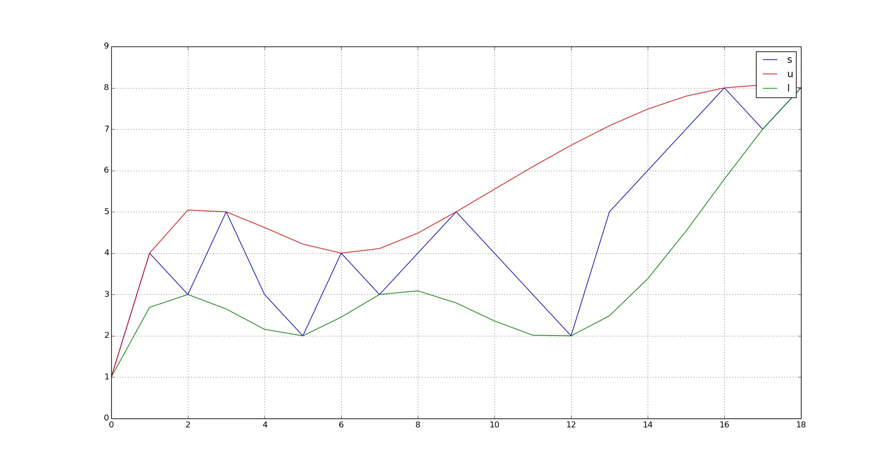
s = array([1,4,3,5,3,2,4,3,4,5,4,3,2,5,6,7,8,7,8]) #This is your noisy vector of values.

q_u = zeros(s.shape)
q_l = zeros(s.shape)

#Prepend the first value of (s) to the interpolating values. This forces the model to use the same starting point for both the upper and lower envelope models.

u_x = [0,]
u_y = [s[0],]

l_x = [0,]
l_y = [s[0],]

#Detect peaks and troughs and mark their location in u_x,u_y,l_x,l_y respectively.

for k in xrange(1,len(s)-1):
    if (sign(s[k]-s[k-1])==1) and (sign(s[k]-s[k+1])==1):
        u_x.append(k)
        u_y.append(s[k])

    if (sign(s[k]-s[k-1])==-1) and ((sign(s[k]-s[k+1]))==-1):
        l_x.append(k)
        l_y.append(s[k])

#Append the last value of (s) to the interpolating values. This forces the model to use the same ending point for both the upper and lower envelope models.

u_x.append(len(s)-1)
u_y.append(s[-1])

l_x.append(len(s)-1)
l_y.append(s[-1])

#Fit suitable models to the data. Here I am using cubic splines, similarly to the MATLAB example given in the question.

u_p = interp1d(u_x,u_y, kind = 'cubic',bounds_error = False, fill_value=0.0)
l_p = interp1d(l_x,l_y,kind = 'cubic',bounds_error = False, fill_value=0.0)

#Evaluate each model over the domain of (s)
for k in xrange(0,len(s)):
    q_u[k] = u_p(k)
    q_l[k] = l_p(k)

#Plot everything
plot(s);hold(True);plot(q_u,'r');plot(q_l,'g');grid(True);show()

这会产生以下输出：

进一步改进的要点：

1. 上述代码未过滤可能发生在某个阈值“距离”（如时间）内的峰值或谷值。这类似于envelope的第二个参数。然而，通过检查u_x,u_y连续值之间的差异来轻松添加它。

2. 然而，先使用移动平均滤波器对数据进行低通滤波可以快速改善前面提到的问题，然后再插值上下包络函数。您可以通过将（s）与适当的移动平均滤波器卷积来轻松实现此操作。不在此处详细介绍（如果需要可以提供），但为了生成一个该滤波器可以对N个连续样本起作用的移动平均滤波器，您可以执行以下操作：s_filtered = numpy.convolve(s, numpy.ones((1,N))/float(N) 。 （N）越高，您的数据看起来就越平稳。请注意，由于称为group delay的平滑滤波器的原因，在s_filtered中，这将使（s）值向右移动（N/2）个样本。有关移动平均值的更多信息，请参见this link 。

希望这能有所帮助。 （如果提供了原始应用程序的更多信息，我很乐意修改回复。也许数据可以以更合适的方式进行预处理（？））

- A_A

---

非常感谢你提供这么详细的答复！是的，我一直在寻找某种形式的滤波器（中值等）来帮助平滑数据。我的数据来自分子动力学，所以比你的例子要嘈杂得多，但我一定会尝试一下！ - user5224720

很高兴听到它有所帮助。一个关于你的数据示例的图表可能也会有所帮助。从分子动力学的角度来看，这个信号反映了什么？ - A_A

Answer 3

在@A_A的回答基础上，将符号检查替换为nim/max测试，使其更加健壮。最初的回答：

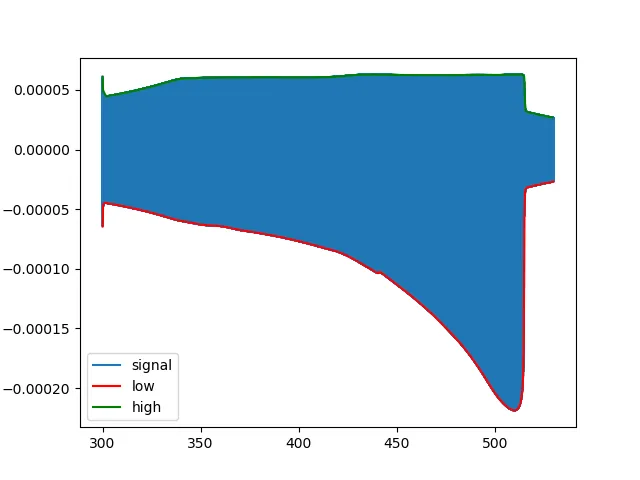
在@A_A的回答基础上，用nim/max测试来代替符号检查，使代码更加健壮。

import numpy as np
import scipy.interpolate
import matplotlib.pyplot as pt
%matplotlib inline

t = np.multiply(list(range(1000)), .1)
s = 10*np.sin(t)*t**.5

u_x = [0]
u_y = [s[0]]

l_x = [0]
l_y = [s[0]]

#Detect peaks and troughs and mark their location in u_x,u_y,l_x,l_y respectively.
for k in range(2,len(s)-1):
    if s[k] >= max(s[:k-1]):
        u_x.append(t[k])
        u_y.append(s[k])

for k in range(2,len(s)-1):
    if s[k] <= min(s[:k-1]):
        l_x.append(t[k])
        l_y.append(s[k])

u_p = scipy.interpolate.interp1d(u_x, u_y, kind = 'cubic', bounds_error = False, fill_value=0.0)
l_p = scipy.interpolate.interp1d(l_x, l_y, kind = 'cubic', bounds_error = False, fill_value=0.0)

q_u = np.zeros(s.shape)
q_l = np.zeros(s.shape)
for k in range(0,len(s)):
    q_u[k] = u_p(t[k])
    q_l[k] = l_p(t[k])

pt.plot(t,s)
pt.plot(t, q_u, 'r')
pt.plot(t, q_l, 'g')

如果你期望函数是递增的，请尝试：

最初的回答：

for k in range(1,len(s)-2):
    if s[k] <= min(s[k+1:]):
        l_x.append(t[k])
        l_y.append(s[k])

最初的回答：

用于下凸壳。

- mousomer

Answer 4

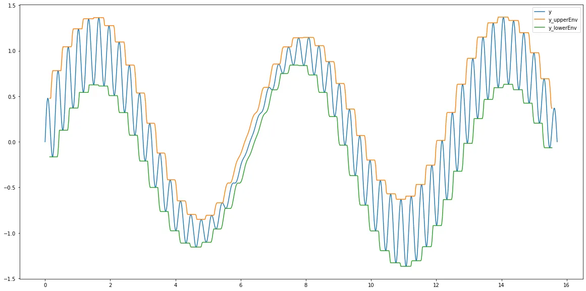
或者您可以使用pandas。这里我只需要两行代码：

import pandas as pd
import numpy as np


x=np.linspace(0,5*np.pi,1000)
y=np.sin(x)+0.4*np.cos(x/4)*np.sin(x*20)

df=pd.DataFrame(data={"y":y},index=x)

windowsize = 20
df["y_upperEnv"]=df["y"].rolling(window=windowsize).max().shift(int(-windowsize/2))
df["y_lowerEnv"]=df["y"].rolling(window=windowsize).min().shift(int(-windowsize/2))

df.plot(figsize=(20,10))

Output:

- MSt Engineering

Answer 5

我发现使用scipy函数的组合比其他方法表现更好。

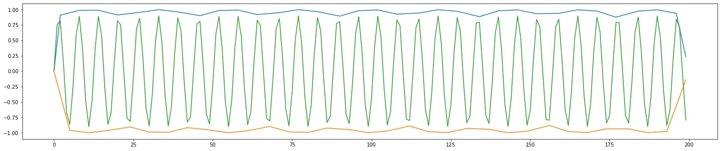
def envelope(sig, distance):
    # split signal into negative and positive parts
    u_x = np.where(sig > 0)[0]
    l_x = np.where(sig < 0)[0]
    u_y = sig.copy()
    u_y[l_x] = 0
    l_y = -sig.copy()
    l_y[u_x] = 0
    
    # find upper and lower peaks
    u_peaks, _ = scipy.signal.find_peaks(u_y, distance=distance)
    l_peaks, _ = scipy.signal.find_peaks(l_y, distance=distance)
    
    # use peaks and peak values to make envelope
    u_x = u_peaks
    u_y = sig[u_peaks]
    l_x = l_peaks
    l_y = sig[l_peaks]
    
    # add start and end of signal to allow proper indexing
    end = len(sig)
    u_x = np.concatenate((u_x, [0, end]))
    u_y = np.concatenate((u_y, [0, 0]))
    l_x = np.concatenate((l_x, [0, end]))
    l_y = np.concatenate((l_y, [0, 0]))
    
    # create envelope functions
    u = scipy.interpolate.interp1d(u_x, u_y)
    l = scipy.interpolate.interp1d(l_x, l_y)
    return u, l

def test():
    x = np.arange(200)
    sig = np.sin(x)
    u, l = envelope(sig, 1)
    
    plt.figure(figsize=(25,5))
    plt.plot(x, u(x))
    plt.plot(x, l(x))
    plt.plot(x, sig*0.9)
    plt.show()
    
test()

- Rijul Gupta

Answer 6

你可能需要查看希尔伯特变换，这很可能是MATLAB中包络函数背后的实际代码。scipy的信号子模块具有内置的希尔伯特变换，并且文档中有一个不错的示例，其中提取了振荡信号的包络： https://docs.scipy.org/doc/scipy/reference/generated/scipy.signal.hilbert.html

- JMK