我希望知道一个绘制度分布图表的脚本输出是否正确。
这个脚本是这样的(向量包含所有顶点度数的向量存储在x中):
x 是:
我的问题是,似乎Log-Log图不正确——例如,我总共有8个“7”度数,那么在Log-Log图上,这个点不应该成为0.845(log 7) / 0.903 (log(8)如(x/y)所示吗?
此外,有人可以告诉我如何将线(对数-对数比例上的幂律)拟合到屏幕2中的图形上吗?
这个脚本是这样的(向量包含所有顶点度数的向量存储在x中):
x 是:
x
 [1] 7 9 8 5 6 2 8 9 7 5 2 4 6 9 2 6 10 8
x是某个网络顶点的度数 - 就像顶点1的度数为7,顶点2的度数为9等等。 x <- v2 summary(x)
x是一个变量,被赋值为v2的值。summary(x)会显示x的统计摘要信息。library(igraph)
split.screen(c(1,2))
screen(1)
plot (tabulate(x), log = "xy", ylab = "Frequency (log scale)", xlab = "Degree (log scale)", main = "Log-log plot of degree distribution")
screen(2)
y <- (length(x) - rank(x, ties.method = "first"))/length(x)
plot(x, y, log = "xy", ylab = "Fraction with min. degree k (log scale)", xlab = "Degree (k) (log scale)", main = "Cumulative log-log plot of degree distribution")
close.screen(all = TRUE)
power.law.fit(x, xmin = 50)
我的问题是,似乎Log-Log图不正确——例如,我总共有8个“7”度数,那么在Log-Log图上,这个点不应该成为0.845(log 7) / 0.903 (log(8)如(x/y)所示吗?
此外,有人可以告诉我如何将线(对数-对数比例上的幂律)拟合到屏幕2中的图形上吗?