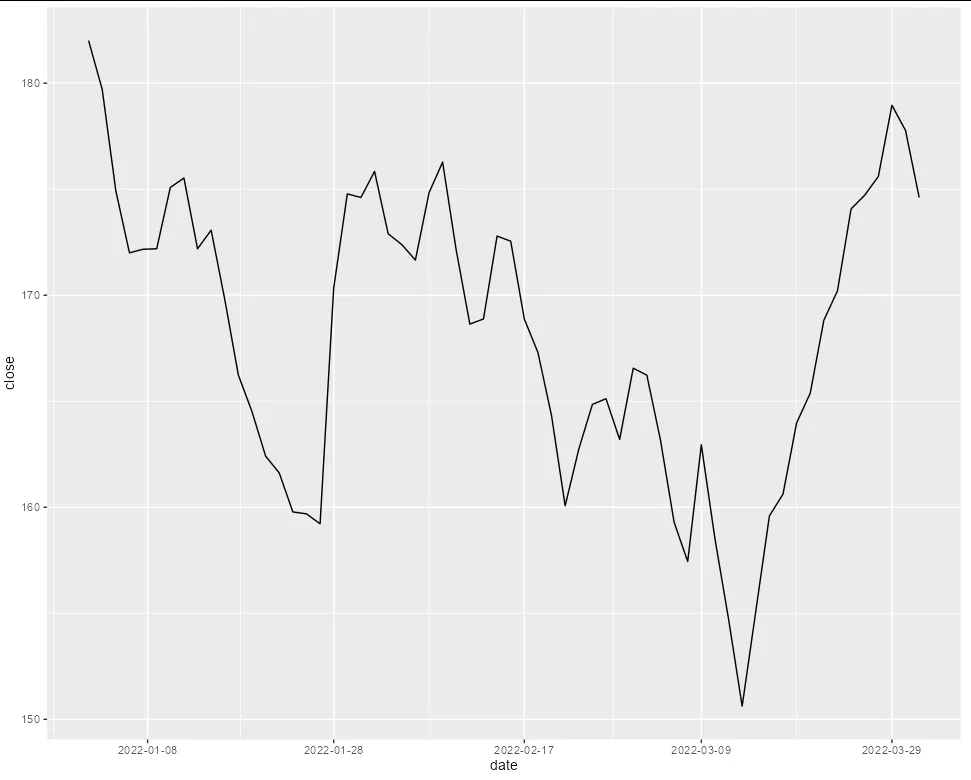
为了在ggplot中摆脱非交易日(即周末)的影响,我使用数据中的行数来代替日期,并添加间隔和标签。下面的代码 "works" 可以实现这一目的,并画出 quantmod 包中的 chartSeries 数据图。
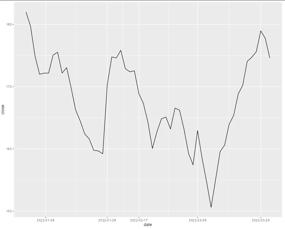
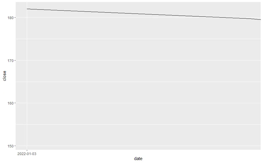
但由于这只是一个标签问题,使用轴转换函数会更加逻辑清晰和简单易用。我尝试创建一个scale_x_finance函数(见 does not work 部分),但我可能误解了反函数的含义,因为我只得到了一个日期而非整个时间序列的情况。
我阅读了多篇Stack Overflow的问题,例如这个 和这个 ,但目前还没有找到解决方法。
我知道存在一个叫做
使用
我在问题底部添加了一些测试数据。
ggplot 会根据绘制的图表类型添加本不存在的信息或显示空白。对于处理股票价格这样的问题不方便。因此,works 部分可以解决该问题。但由于这只是一个标签问题,使用轴转换函数会更加逻辑清晰和简单易用。我尝试创建一个scale_x_finance函数(见 does not work 部分),但我可能误解了反函数的含义,因为我只得到了一个日期而非整个时间序列的情况。
我阅读了多篇Stack Overflow的问题,例如这个 和这个 ,但目前还没有找到解决方法。
我知道存在一个叫做
bdscale 的包,但它已经超过六年没有更新了,而且它创建的间隔 / 标签并不符合我的需求。使用
scale_x_finance 的结果应该和 works 部分的图表一样。我想知道我漏掉了什么。我在问题底部添加了一些测试数据。
works
library(ggplot2)

# get the start date and the last days of the month for breaks and label positions
get_breaks <- function(x) {
  out <- c(1, which(ave(as.numeric(x),format(x,"%Y%m"), FUN = function(x) x == max(x)) == 1))
}

# use 1:nrow to be able to use scale_x_continuous
ggplot(test_data, aes(x = 1:nrow(test_data))) +
  geom_line(aes(y = close)) +
  scale_x_continuous(name = "date",
                     breaks = get_breaks(test_data$date),
                     labels = test_data$date[get_breaks(test_data$date)])
无法工作
scale_x_finance <- function (...,
                             dates,
                             breaks = get_breaks(dates)){

  my_transformer <- function(dates, breaks = get_breaks(dates)) {

    transform <- function(dates) seq_along(dates)
    inverse <- function(nums) dates[nums]

    scales::trans_new(name = "date",
                      transform = transform,
                      inverse = inverse,
                      breaks = breaks,
                      domain = range(dates))
  }

  scale_x_continuous(name = "date",
                     trans = my_transformer(dates = dates, breaks = breaks),
                     ...)
}


ggplot(test_data, aes(x = date)) +
  geom_line(aes(y = close)) +
  scale_x_finance(dates = test_data$date)
数据:
test_data <- structure(list(date = structure(c(18995, 18996, 18997, 18998,
                                               18999, 19002, 19003, 19004, 19005, 19006, 19010, 19011, 19012,
                                               19013, 19016, 19017, 19018, 19019, 19020, 19023, 19024, 19025,
                                               19026, 19027, 19030, 19031, 19032, 19033, 19034, 19037, 19038,
                                               19039, 19040, 19041, 19045, 19046, 19047, 19048, 19051, 19052,
                                               19053, 19054, 19055, 19058, 19059, 19060, 19061, 19062, 19065,
                                               19066, 19067, 19068, 19069, 19072, 19073, 19074, 19075, 19076,
                                               19079, 19080, 19081, 19082), class = "Date"),
                            close = c(182.009995, 179.699997, 174.919998, 172, 172.169998, 172.190002, 175.080002,
                                      175.529999, 172.190002, 173.070007, 169.800003, 166.229996, 164.509995,
                                      162.410004, 161.619995, 159.779999, 159.690002, 159.220001, 170.330002,
                                      174.779999, 174.610001, 175.839996, 172.899994, 172.389999, 171.660004,
                                      174.830002, 176.279999, 172.119995, 168.639999, 168.880005, 172.789993,
                                      172.550003, 168.880005, 167.300003, 164.320007, 160.070007, 162.740005,
                                      164.850006, 165.119995, 163.199997, 166.559998, 166.229996, 163.169998,
                                      159.300003, 157.440002, 162.949997, 158.520004, 154.729996, 150.619995,
                                      155.089996, 159.589996, 160.619995, 163.979996, 165.380005, 168.820007,
                                      170.210007, 174.070007, 174.720001, 175.600006, 178.960007, 177.770004,
                                      174.610001)), row.names = c(NA, 62L), class = "data.frame")