Python-给定数据集预测/外推未来数据

Question

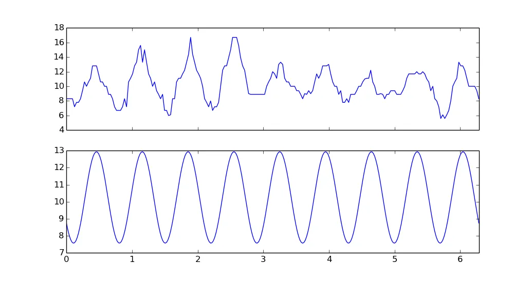
我对Python非常陌生。我有一个数据集，想使用numPy/sciPy来预测/推断未来的数据点。是否有一种简单的方法来得到一个数学函数（比如正弦函数），以使其符合我的当前数据，然后我可以通过这个函数传递新值来获取我的预测结果？

以下是我拥有的内容，但我认为它没有达到我想要的效果：

import numpy as np
from scipy.optimize import curve_fit
import matplotlib.pyplot as plt

def main():

    y = [8.3, 8.3, 8.3, 8.3, 7.2, 7.8, 7.8, 8.3, 9.4, 10.6, 10.0, 10.6, 11.1, 12.8,
         12.8, 12.8, 11.7, 10.6, 10.6, 10.0, 10.0, 8.9, 8.9, 8.3, 7.2, 6.7, 6.7, 6.7,
         7.2, 8.3, 7.2, 10.6, 11.1, 11.7, 12.8, 13.3, 15.0, 15.6, 13.3, 15.0, 13.3,
         11.7, 11.1, 10.0, 10.6, 9.4, 8.9, 8.3, 8.9, 6.7, 6.7, 6.0, 6.1, 8.3, 8.3,
         10.6, 11.1, 11.1, 11.7, 12.2, 13.3, 14.4, 16.7, 14.4, 13.3, 12.2, 11.7,
         11.1, 10.0, 8.3, 7.8, 7.2, 8.0, 6.7, 7.2, 7.2, 7.8, 10.0, 12.2, 12.8,
         12.8, 13.9, 15.0, 16.7, 16.7, 16.7, 15.6, 13.9, 12.8, 12.2, 10.6, 9.0,
         8.9, 8.9, 8.9, 8.9, 8.9, 8.9, 8.9, 8.9, 10.0, 10.6, 11.1, 12.0, 11.7,
         11.1, 13.0, 13.3, 13.0, 11.1, 10.6, 10.6, 10.0, 10.0, 10.0, 9.4, 9.4,
         8.9, 8.3, 9.0, 8.9, 9.4, 9.0, 9.4, 10.6, 11.7, 11.1, 11.7, 12.8, 12.8,
         12.8, 13.0, 11.7, 10.6, 10.0, 10.0, 8.9, 9.4, 7.8, 7.8, 8.3, 7.8, 8.9,
         8.9, 8.9, 9.4, 10.0, 10.0, 10.6, 11.0, 11.1, 11.1, 12.2, 10.6, 10.0, 8.9,
         8.9, 9.0, 8.9, 8.3, 8.9, 8.9, 9.4, 9.4, 9.4, 8.9, 8.9, 8.9, 9.4, 10.0,
         11.1, 11.7, 11.7, 11.7, 11.7, 12.0, 11.7, 11.7, 12.0, 11.7, 11.0, 10.6,
         9.4, 10.0, 8.3, 8.0, 7.2, 5.6, 6.1, 5.6, 6.1, 6.7, 8.0, 10.0, 10.6, 11.1,
         13.3, 12.8, 12.8, 12.2, 11.1, 10.0, 10.0, 10.0, 10.0, 9.4, 8.3]    
    x = np.array(np.arange(len(y)))        

    fitting_parameters, covariance = curve_fit(fit, x, y)
    a = fitting_parameters[0]
    b = fitting_parameters[1]
    c = fitting_parameters[2]
    d = fitting_parameters[3]

    for x_predict in range(len(y) + 1, len(y) + 24):
        next_x = x_predict
        next_y = fit(next_x, a, b, c, d)

        print("next_x: " + str(next_x))
        print("next_y: " + str(next_y))
        y.append(next_y)

    plt.plot(y)
    plt.show()

def fit(x, a, b, c, d):
    return a*np.sin(b*x + c) + d

我尝试使用curve_fit和univariatespline来处理我的数据，但这两种方法只是分别适应了我的当前数据并平滑了我的点。我的问题是，这些工具只是“拟合”了我的数据，而没有给我一个可以用来获取未来数据点的函数。

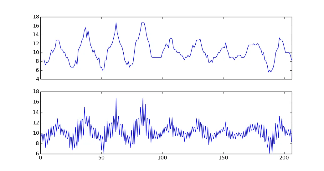
我认为我可以使用离散傅里叶变换，因为我的数据是周期性的，看起来可以描述为正弦和余弦的总和。但是一旦我从时域得到频率域，我就不知道如何进行“外推”，以便预测时间域中的未来周期和数据点。

import numpy as np
import matplotlib.pyplot as plt

mydata = [8.3, 8.3, 8.3, 8.3, 7.2, 7.8, 7.8, 8.3, 9.4, 10.6, 10.0, 10.6, 11.1, 12.8,
         12.8, 12.8, 11.7, 10.6, 10.6, 10.0, 10.0, 8.9, 8.9, 8.3, 7.2, 6.7, 6.7, 6.7,
         7.2, 8.3, 7.2, 10.6, 11.1, 11.7, 12.8, 13.3, 15.0, 15.6, 13.3, 15.0, 13.3,
         11.7, 11.1, 10.0, 10.6, 9.4, 8.9, 8.3, 8.9, 6.7, 6.7, 6.0, 6.1, 8.3, 8.3,
         10.6, 11.1, 11.1, 11.7, 12.2, 13.3, 14.4, 16.7, 14.4, 13.3, 12.2, 11.7,
         11.1, 10.0, 8.3, 7.8, 7.2, 8.0, 6.7, 7.2, 7.2, 7.8, 10.0, 12.2, 12.8,
         12.8, 13.9, 15.0, 16.7, 16.7, 16.7, 15.6, 13.9, 12.8, 12.2, 10.6, 9.0,
         8.9, 8.9, 8.9, 8.9, 8.9, 8.9, 8.9, 8.9, 10.0, 10.6, 11.1, 12.0, 11.7,
         11.1, 13.0, 13.3, 13.0, 11.1, 10.6, 10.6, 10.0, 10.0, 10.0, 9.4, 9.4,
         8.9, 8.3, 9.0, 8.9, 9.4, 9.0, 9.4, 10.6, 11.7, 11.1, 11.7, 12.8, 12.8,
         12.8, 13.0, 11.7, 10.6, 10.0, 10.0, 8.9, 9.4, 7.8, 7.8, 8.3, 7.8, 8.9,
         8.9, 8.9, 9.4, 10.0, 10.0, 10.6, 11.0, 11.1, 11.1, 12.2, 10.6, 10.0, 8.9,
         8.9, 9.0, 8.9, 8.3, 8.9, 8.9, 9.4, 9.4, 9.4, 8.9, 8.9, 8.9, 9.4, 10.0,
         11.1, 11.7, 11.7, 11.7, 11.7, 12.0, 11.7, 11.7, 12.0, 11.7, 11.0, 10.6,
         9.4, 10.0, 8.3, 8.0, 7.2, 5.6, 6.1, 5.6, 6.1, 6.7, 8.0, 10.0, 10.6, 11.1,
         13.3, 12.8, 12.8, 12.2, 11.1, 10.0, 10.0, 10.0, 10.0, 9.4, 8.3] 

sp = np.fft.rfft(mydata)
freq = np.fft.rfftfreq(len(mydata), d= 1.0)

plt.subplot(211)
plt.plot(mydata)
plt.subplot(212)
plt.plot(freq, sp, 'r')
plt.show()

我知道外推可能是危险和不可靠的，但是为了这个项目的目的，我只是想得到一个可以绘制函数图形的工作预测功能。

非常感谢您的帮助。

- ccheng21

---

提供数据图表和代码示例可能会帮助别人帮助你。这也可能不是正确的网站。有一个统计学网站stats.stackexchange.com可能更适合。无论哪种方式，您都需要向人们展示一些样本数据和您用于适配它的一些代码。 - Paul

@Paul 谢谢。我已经添加了一些代码，想要发布一个图表，但我的声望还不够高。 - ccheng21

@unutbu 请检查我添加的第二段代码，其中使用了numpy.fft。我知道我可以在频域上使用逆rfft函数返回到时间域，但我首先需要以某种方式操作我的频率数据以获取预测值...这就是我卡住的地方。谢谢！ - ccheng21

你的第一个代码示例永远无法适应数据，因为它假设振幅是恒定的。像第二个示例中使用傅里叶分解可以提供变化的振幅。要进行一些外推，您需要有一些想法，您希望函数看起来像什么，或者使用一些机器学习技术，但这两个主题都不在此讨论范围内，您可能想尝试http://stats.stackexchange.com。 - Benjamin Bannier

适用于http://stats.stackexchange.com - Benjamin Bannier

Answer 1

这里有一种插值方法，可以将您的周期性数据表示为傅里叶级数。傅里叶级数中使用的系数是通过离散FFT获得的。

我不建议这样做--您可以看到下面的插值不是直觉上认为的非常好--但由于我在评论中提到了它，我会继续展示一些代码 :)

import numpy as np
import matplotlib.pyplot as plt
import scipy.fftpack as fftpack

def fft_inverse(Yhat, x):
    """Based on https://dev59.com/QFLTa4cB1Zd3GeqPcq9m#4452499 (mtrw)"""
    Yhat = np.asarray(Yhat)
    x = np.asarray(x).reshape(-1, 1)
    N = len(Yhat)
    k = np.arange(N)
    total = Yhat * np.exp(1j * x * k * 2 * np.pi / N)
    return np.real(total.sum(axis=1))/N

mydata = [8.3, 8.3, 8.3, 8.3, 7.2, 7.8, 7.8, 8.3, 9.4, 10.6, 10.0, 10.6, 11.1, 12.8,
         12.8, 12.8, 11.7, 10.6, 10.6, 10.0, 10.0, 8.9, 8.9, 8.3, 7.2, 6.7, 6.7, 6.7,
         7.2, 8.3, 7.2, 10.6, 11.1, 11.7, 12.8, 13.3, 15.0, 15.6, 13.3, 15.0, 13.3,
         11.7, 11.1, 10.0, 10.6, 9.4, 8.9, 8.3, 8.9, 6.7, 6.7, 6.0, 6.1, 8.3, 8.3,
         10.6, 11.1, 11.1, 11.7, 12.2, 13.3, 14.4, 16.7, 14.4, 13.3, 12.2, 11.7,
         11.1, 10.0, 8.3, 7.8, 7.2, 8.0, 6.7, 7.2, 7.2, 7.8, 10.0, 12.2, 12.8,
         12.8, 13.9, 15.0, 16.7, 16.7, 16.7, 15.6, 13.9, 12.8, 12.2, 10.6, 9.0,
         8.9, 8.9, 8.9, 8.9, 8.9, 8.9, 8.9, 8.9, 10.0, 10.6, 11.1, 12.0, 11.7,
         11.1, 13.0, 13.3, 13.0, 11.1, 10.6, 10.6, 10.0, 10.0, 10.0, 9.4, 9.4,
         8.9, 8.3, 9.0, 8.9, 9.4, 9.0, 9.4, 10.6, 11.7, 11.1, 11.7, 12.8, 12.8,
         12.8, 13.0, 11.7, 10.6, 10.0, 10.0, 8.9, 9.4, 7.8, 7.8, 8.3, 7.8, 8.9,
         8.9, 8.9, 9.4, 10.0, 10.0, 10.6, 11.0, 11.1, 11.1, 12.2, 10.6, 10.0, 8.9,
         8.9, 9.0, 8.9, 8.3, 8.9, 8.9, 9.4, 9.4, 9.4, 8.9, 8.9, 8.9, 9.4, 10.0,
         11.1, 11.7, 11.7, 11.7, 11.7, 12.0, 11.7, 11.7, 12.0, 11.7, 11.0, 10.6,
         9.4, 10.0, 8.3, 8.0, 7.2, 5.6, 6.1, 5.6, 6.1, 6.7, 8.0, 10.0, 10.6, 11.1,
         13.3, 12.8, 12.8, 12.2, 11.1, 10.0, 10.0, 10.0, 10.0, 9.4, 8.3] 

Yhat = fftpack.fft(mydata)

fig, ax = plt.subplots(nrows=2, sharex=True)
xs = np.arange(len(mydata))
ax[0].plot(xs, mydata)

new_xs = np.linspace(xs.min(), xs.max(), len(mydata)*1.5)
new_ys = fft_inverse(Yhat, new_xs)
ax[1].plot(new_xs, new_ys)

plt.xlim(xs.min(), xs.max())
plt.show()

---

以下是使用scipy.optimize查找参数以拟合模型函数的方法，然后可以在任意x坐标处进行插值。尽管使用单个sin进行拟合效果仍然很糟糕，但我将发布代码，只是为了展示如何使用scipy.optimize：

import numpy as np
import matplotlib.pyplot as plt
import scipy.optimize as optimize

mydata = np.array(
    [8.3, 8.3, 8.3, 8.3, 7.2, 7.8, 7.8, 8.3, 9.4, 10.6, 10.0, 10.6, 11.1, 12.8,
     12.8, 12.8, 11.7, 10.6, 10.6, 10.0, 10.0, 8.9, 8.9, 8.3, 7.2, 6.7, 6.7, 6.7,
     7.2, 8.3, 7.2, 10.6, 11.1, 11.7, 12.8, 13.3, 15.0, 15.6, 13.3, 15.0, 13.3,
     11.7, 11.1, 10.0, 10.6, 9.4, 8.9, 8.3, 8.9, 6.7, 6.7, 6.0, 6.1, 8.3, 8.3,
     10.6, 11.1, 11.1, 11.7, 12.2, 13.3, 14.4, 16.7, 14.4, 13.3, 12.2, 11.7,
     11.1, 10.0, 8.3, 7.8, 7.2, 8.0, 6.7, 7.2, 7.2, 7.8, 10.0, 12.2, 12.8,
     12.8, 13.9, 15.0, 16.7, 16.7, 16.7, 15.6, 13.9, 12.8, 12.2, 10.6, 9.0,
     8.9, 8.9, 8.9, 8.9, 8.9, 8.9, 8.9, 8.9, 10.0, 10.6, 11.1, 12.0, 11.7,
     11.1, 13.0, 13.3, 13.0, 11.1, 10.6, 10.6, 10.0, 10.0, 10.0, 9.4, 9.4,
     8.9, 8.3, 9.0, 8.9, 9.4, 9.0, 9.4, 10.6, 11.7, 11.1, 11.7, 12.8, 12.8,
     12.8, 13.0, 11.7, 10.6, 10.0, 10.0, 8.9, 9.4, 7.8, 7.8, 8.3, 7.8, 8.9,
     8.9, 8.9, 9.4, 10.0, 10.0, 10.6, 11.0, 11.1, 11.1, 12.2, 10.6, 10.0, 8.9,
     8.9, 9.0, 8.9, 8.3, 8.9, 8.9, 9.4, 9.4, 9.4, 8.9, 8.9, 8.9, 9.4, 10.0,
     11.1, 11.7, 11.7, 11.7, 11.7, 12.0, 11.7, 11.7, 12.0, 11.7, 11.0, 10.6,
     9.4, 10.0, 8.3, 8.0, 7.2, 5.6, 6.1, 5.6, 6.1, 6.7, 8.0, 10.0, 10.6, 11.1,
     13.3, 12.8, 12.8, 12.2, 11.1, 10.0, 10.0, 10.0, 10.0, 9.4, 8.3]) 


def fit(x, a, b, c, d):
    return a*np.sin(b*x + c) + d

xs = np.linspace(0, 2*np.pi, len(mydata))

guess = (mydata.ptp()/2, 10, 0, mydata.mean())
fitting_parameters, covariance = optimize.curve_fit(fit, xs, mydata, p0=guess)
a, b, c, d = fitting_parameters
print(a, b, c, d)

fig, ax = plt.subplots(nrows=2, sharex=True)
ax[0].plot(xs, mydata)

new_xs = np.linspace(xs.min(), xs.max(), len(mydata)*1.5)
new_ys = fit(new_xs, a, b, c, d)
ax[1].plot(new_xs, new_ys)

plt.xlim(xs.min(), xs.max())
plt.show()

通过选择更好的模型函数（而不是fit），您可以改善拟合效果。选择什么模型取决于创造力和直觉，这些直觉由您对问题领域的先验知识所指导。更好的选择不仅取决于拟合度的好坏，还取决于您希望模型有多简单或复杂，以及/或者应用于新数据集时具有多少预测能力。

- unutbu

---

通过泰勒展开式，多项式可能作为指定域上的拟合函数。 - user7345804