如何解释神经网络回归的多输出回归图？

Question

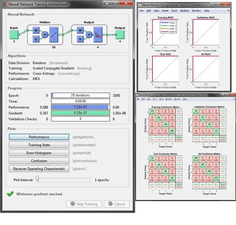
我已经使用MATLAB NN工具箱训练了我的神经网络模型。 我的网络有多个输入和多个输出，分别为6和7。基于此，我想澄清几个问题：

• 训练结束时显示的最终回归图显示很好的精度，R〜0.99。 但是，由于我有多个输出，我不确定它代表哪个散点图？ 难道我们不应该为每个输出变量拥有7个目标与预测图？

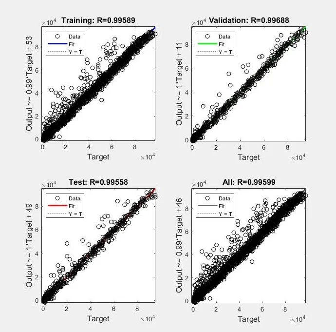
• 据我所知，R ^ 2是评论模型准确性更好的方法，而MATLAB在其图中报告R。 我将该R作为R ^ 2处理还是应该对报告的R值进行平方以获得R ^ 2。
• 我已生成包含权重、偏差和激活函数的Matlab脚本，作为训练的最终结果。 因此，我是否能够简单地将原始数据作为输入并获得相应的预测输出。 我使用Matlab选择用于训练的索引提供了完全相同的训练集（以进行交叉检验），并绘制了预测的输出与实际输出，但结果一点也不好。 明显，不符合R〜0.99的标准。 我做错了什么吗？

代码：

function [y1] = myNeuralNetworkFunction_2(x1)
%MYNEURALNETWORKFUNCTION neural network simulation function.
% X = [torque T_exh lambda t_Spark N EGR];
% Y = [O2R CO2R HC NOX CO lambda_out T_exh2];
% Generated by Neural Network Toolbox function genFunction, 17-Dec-2018 07:13:04.
%
% [y1] = myNeuralNetworkFunction(x1) takes these arguments:
%   x = Qx6 matrix, input #1
% and returns:
%   y = Qx7 matrix, output #1
% where Q is the number of samples.

%#ok<*RPMT0>

% ===== NEURAL NETWORK CONSTANTS =====

% Input 1
x1_step1_xoffset = [-24;235.248;0.75;-20.678;550;0.799];
x1_step1_gain = [0.00353982300884956;0.00284355877067267;6.26959247648903;0.0275865874012055;0.000366568914956012;0.0533831576137729];
x1_step1_ymin = -1;

% Layer 1
b1 = [1.3808996210168685;-2.0990163849711894;0.9651733083552595;0.27000953282929346;-1.6781835509820286;-1.5110463684800366;-3.6257438832309905;2.1569498669085361;1.9204156230460485;-0.17704342477904209];
IW1_1 = [-0.032892214008082517 -0.55848270745152429 -0.0063993424771670616 -0.56161004933654057 2.7161844536020197 0.46415317073346513;-0.21395624254052176 -3.1570133640176681 0.71972178875396853 -1.9132557838515238 1.3365248285282931 -3.022721627052706;-1.1026780445896862 0.2324603066452392 0.14552308208231421 0.79194435276493658 -0.66254679969168417 0.070353201192052434;-0.017994515838487352 -0.097682677816992206 0.68844109281256027 -0.001684535122025588 0.013605622123872989 0.05810686279306107;0.5853667840629273 -2.9560683084876329 0.56713425120259764 -2.1854386350040116 1.2930115031659106 -2.7133159265497957;0.64316656469750333 -0.63667017646313084 0.50060179040086761 -0.86827897068177973 2.695456517458648 0.16822164719859456;-0.44666821007466739 4.0993786464616679 -0.89370838440321498 3.0445073606237933 -3.3015566360833453 -4.492874075961689;1.8337574137485424 2.6946232855369989 1.1140472073136622 1.6167763205944321 1.8573696127039145 -0.81922672766933646;-0.12561950922781362 3.0711045035224349 -0.6535751823440773 2.0590707752473199 -1.3267693770634292 2.8782780742777794;-0.013438026967107483 -0.025741311825949621 0.45460734966889638 0.045052447491038108 -0.21794568374100454 0.10667240367191703];

% Layer 2
b2 = [-0.96846557414356171;-0.2454718918618051;-0.7331628718025488;-1.0225195290982099;0.50307202195645395;-0.49497234988401961;-0.21817117469133171];
LW2_1 = [-0.97716474643411022 -0.23883775971686808 0.99238069915206006 0.4147649511973347 0.48504023209224734 -0.071372217431684551 0.054177719330469304 -0.25963474838320832 0.27368380212104881 0.063159321947246799;-0.15570858147605909 -0.18816739764334323 -0.3793600124951475 2.3851961990944681 0.38355142531334563 -0.75308427071748985 -0.1280128732536128 -1.361052031781103 0.6021878865831336 -0.24725687748503239;0.076251356114485525 -0.10178293627600112 0.10151304376762409 -0.46453434441403058 0.12114876632815359 0.062856969143306296 -0.0019628163322658364 -0.067809039768745916 0.071731544062023825 0.65700427778446913;0.17887084584125315 0.29122649575978238 0.37255802759192702 1.3684190468992126 0.60936238465090853 0.21955911453674043 0.28477957899364675 -0.051456306721251184 0.6519451272106177 -0.64479205028051967;0.25743349663436799 2.0668075180209979 0.59610776847961111 -3.2609682919282603 1.8824214917530881 0.33542869933904396 0.03604272669356564 -0.013842766338427388 3.8534510207741826 2.2266745660915586;-0.16136175574939746 0.10407287099228898 -0.13902245286490234 0.87616472446622717 -0.027079111747601223 0.024812287505204988 -0.030101536834009103 0.043168268669541855 0.12172932035587079 -0.27074383434206573;0.18714562505165402 0.35267726325386606 -0.029241400610813449 0.53053853235049087 0.58880054832728757 0.047959541165126809 0.16152268183097709 0.23419456403348898 0.83166785128608967 -0.66765237856750781];

% Output 1
y1_step1_ymin = -1;
y1_step1_gain = [0.114200879346771;0.145581598485951;0.000139011547272197;0.000456244862967996;2.05816254143146e-05;5.27704485488127;0.00284355877067267];
y1_step1_xoffset = [-0.045;1.122;2.706;17.108;493.726;0.75;235.248];

% ===== SIMULATION ========

% Dimensions
Q = size(x1,1); % samples

% Input 1
x1 = x1';
xp1 = mapminmax_apply(x1,x1_step1_gain,x1_step1_xoffset,x1_step1_ymin);

% Layer 1
a1 = tansig_apply(repmat(b1,1,Q) + IW1_1*xp1);

% Layer 2
a2 = repmat(b2,1,Q) + LW2_1*a1;

% Output 1
y1 = mapminmax_reverse(a2,y1_step1_gain,y1_step1_xoffset,y1_step1_ymin);
y1 = y1';
end

% ===== MODULE FUNCTIONS ========

% Map Minimum and Maximum Input Processing Function
function y = mapminmax_apply(x,settings_gain,settings_xoffset,settings_ymin)
y = bsxfun(@minus,x,settings_xoffset);
y = bsxfun(@times,y,settings_gain);
y = bsxfun(@plus,y,settings_ymin);
end

% Sigmoid Symmetric Transfer Function
function a = tansig_apply(n)
a = 2 ./ (1 + exp(-2*n)) - 1;
end

% Map Minimum and Maximum Output Reverse-Processing Function
function x = mapminmax_reverse(y,settings_gain,settings_xoffset,settings_ymin)
x = bsxfun(@minus,y,settings_ymin);
x = bsxfun(@rdivide,x,settings_gain);
x = bsxfun(@plus,x,settings_xoffset);
end

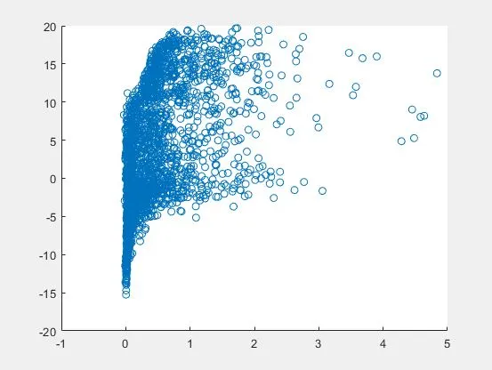
以上是自动生成的代码。我用来交叉检查第一个变量的绘图如下：

% X and Y are input and output - same as above
X_train = X(results.info1.train.indices,:);
y_train = Y(results.info1.train.indices,:);
out_train = myNeuralNetworkFunction_2(X_train);
scatter(y_train(:,1),out_train(:,1))

- Manish

---

你使用的NN工具箱版本是什么？如果我没记错，最新版本更名为“深度学习工具箱”。只是想澄清一下，你是说模型脚本是由NN工具箱中的某个函数自动生成的，用于生成预测吗？ - Margaret Schrayer

Answer 1

回答你关于R的问题：是的，你应该平方R以获取R^2值。在这种情况下，它们将非常接近，因为R非常接近1。

- Margaret Schrayer

Answer 2

首先，您要解决的问题是回归问题吗？还是将7个类转换为数字的分类问题？我假设这是一个分类问题，因为您正在尝试获取每个类的成功率。

至于您的第一个问题：根据文献，建议使用值"All: R"。如果您想获得每个类的成功率，需要达到分类问题中有效的精度、召回率、F-度量、FP率、TP率等值。有许多Matlab文档可供参考（帮助ROC），您可以查看详细信息。我提到的所有值，以及我认为您实际想要的所有值，都可以从混淆矩阵中获得。

这方面有一个很好的例子。

[x,t] = simpleclass_dataset;
net = patternnet(10);
net = train(net,x,t);
y = net(x);
[c,cm,ind,per] = confusion(t,y)

希望您在运行代码时看到的“nntraintool”窗口中找到所需内容。

你的其他问题已经得到了回答。或者，你可以考虑使用像Weka这样的开源软件来使用机器学习算法。

- NCC1701

Answer 3

这些图表显示了估计值和真实（目标）值之间的相关性。因此，R是相关性的强度。您可以将其平方以找到R平方。

您绘制的图形和Matlab给出的图形不是相同变量的图形。轴的范围或比例尺非常不同。

- Ipek DK