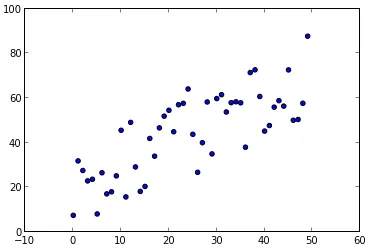
假设我有一组随机的X,Y点:
x = np.array(range(0,50))
y = np.random.uniform(low=0.0, high=40.0, size=200)
y = map((lambda a: a[0] + a[1]), zip(x,y))
plt.scatter(x,y)
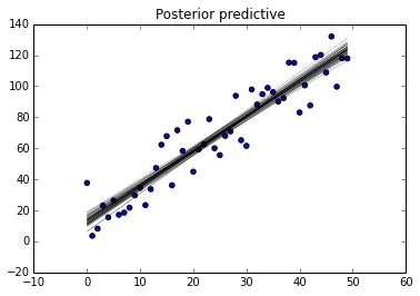
y建模为每个x值的高斯分布,我该如何估计后验预测,即每个(可能的)x值的p(y|x)?是否可以使用pymc或scikit-learn轻松实现此操作?假设我有一组随机的X,Y点:
x = np.array(range(0,50))
y = np.random.uniform(low=0.0, high=40.0, size=200)
y = map((lambda a: a[0] + a[1]), zip(x,y))
plt.scatter(x,y)
y建模为每个x值的高斯分布,我该如何估计后验预测,即每个(可能的)x值的p(y|x)?是否可以使用pymc或scikit-learn轻松实现此操作?import numpy as np
import pymc as pm
import matplotlib.pyplot as plt
from pymc import glm
## Make some data
x = np.array(range(0,50))
y = np.random.uniform(low=0.0, high=40.0, size=50)
y = 2*x+y
## plt.scatter(x,y)
data = dict(x=x, y=y)
with pm.Model() as model:
# specify glm and pass in data. The resulting linear model, its likelihood and
# and all its parameters are automatically added to our model.
pm.glm.glm('y ~ x', data)
step = pm.NUTS() # Instantiate MCMC sampling algorithm
trace = pm.sample(2000, step)
##fig = pm.traceplot(trace, lines={'alpha': 1, 'beta': 2, 'sigma': .5});## traces
fig = plt.figure()
ax = fig.add_subplot(111)
plt.scatter(x, y, label='data')
glm.plot_posterior_predictive(trace, samples=50, eval=x,
label='posterior predictive regression lines')
 ,您可能会对以下博客文章感兴趣:1和2。这些博客是我从中汲取灵感的。
编辑
要获取每个x的y值,请尝试使用我从glm源代码中挖掘出来的方法。
,您可能会对以下博客文章感兴趣:1和2。这些博客是我从中汲取灵感的。
编辑
要获取每个x的y值,请尝试使用我从glm源代码中挖掘出来的方法。lm = lambda x, sample: sample['Intercept'] + sample['x'] * x ## linear model
samples=50 ## Choose to be the same as in plot call
trace_det = np.empty([samples, len(x)]) ## initialise
for i, rand_loc in enumerate(np.random.randint(0, len(trace), samples)):
rand_sample = trace[rand_loc]
trace_det[i] = lm(x, rand_sample)
y = trace_det.T
y[0]
如果这不是最优雅的写法,我很抱歉 - 希望您能够理解其中的逻辑。
y[0],y[1],... y[50]的样本(即每个y[i]的样本向量)。你知道我怎么能得到它吗? - Amelio Vazquez-Reina