我相信可以通过创建自定义模型公式及其梯度的函数来实现此事。标准的SSlogis函数使用以下形式的逻辑函数:
f(input) = Asym/(1+exp((xmid-input)/scal)) # as in ?SSlogis
不必调用SSlogis,您可以修改上述语句以适应您的需求。我相信您希望查看性别是否对固定效应产生影响。以下是修改Asym2中特定性别Asym亚群效应的示例代码:
library(nlme)
library(lme4)
Model <- function(age, Asym, Asym2, xmid, scal, Gender)
{
(Asym+Asym2*Gender)/(1+exp((xmid-age)/scal))
}
ModelGradient <- deriv(
body(Model)[[2]],
namevec = c("Asym", "Asym2", "xmid", "scal"),
function.arg=Model
)
引入性别效应的一种相对典型的方法是使用二进制编码。我将把Sex变量转换为一个二进制编码的Gender:
Orthodont2 <- data.frame(Orthodont, Gender = as.numeric(Orthodont[,"Sex"])-1)
Orthodont2 <- Orthodont2[order(Orthodont2[,"Subject"]),]
我可以使用定制模型进行拟合:
fit <- nlmer(
distance ~
ModelGradient(age = age, Asym, Asym2, xmid, scal, Gender = Gender) ~
(Asym | Subject) + (xmid | Subject),
data = Orthodont2,
start = c(Asym = 25, Asym2 = 15, xmid = 11, scal = 3))
当
性别==0(男性)时,模型会达到以下值:
(Asym+Asym2*0)/(1+exp((xmid-age)/scal)) = (Asym)/(1+exp((xmid-age)/scal))
这实际上是标准的SSlogis函数形式。然而,现在有一个二进制开关,如果Gender==1(女性):
(Asym+Asym2)/(1+exp((xmid-age)/scal))
当年龄增长时,女性个体实际达到的渐近水平是Asym + Asym2,而不仅仅是Asym。
请注意,我没有为Asym2指定新的随机效应。因为Asym对于性别来说并不具体,所以女性个体也可能由于Asym项而具有其个体渐近水平的方差。模型拟合:
> summary(fit)
Nonlinear mixed model fit by the Laplace approximation
Formula: distance ~ ModelGradient(age = age, Asym, Asym2, xmid, scal,      Gender = Gender) ~ (Asym | Subject) + (xmid | Subject)
   Data: Orthodont2
   AIC   BIC logLik deviance
 268.7 287.5 -127.4    254.7
Random effects:
 Groups   Name Variance Std.Dev.
 Subject  Asym 7.0499   2.6552
 Subject  xmid 4.4285   2.1044
 Residual      1.5354   1.2391
Number of obs: 108, groups: Subject, 27

Fixed effects:
      Estimate Std. Error t value
Asym    29.882      1.947  15.350
Asym2   -3.493      1.222  -2.859
xmid     1.240      1.068   1.161
scal     5.532      1.782   3.104

Correlation of Fixed Effects:
      Asym   Asym2  xmid
Asym2 -0.471
xmid  -0.584  0.167
scal   0.901 -0.239 -0.773
看起来可能存在性别特异性影响(t值为-2.859),因此随着年龄的增长,女性患者似乎会达到稍低的“距离”值:29.882-3.493 = 26.389。
我并不一定认为这是一个好/最佳模型,只是展示了如何通过自定义 lme4 中的非线性模型进行进一步操作。如果您想提取非线性固定效应的可视化效果(类似于在如何按观察值提取lmer固定效应?中线性模型的可视化效果),则需要进行一些调整。
fixefmat <- matrix(rep(fixef(fit), times=dim(Orthodont2)[1]), ncol=length(fixef(fit)), byrow=TRUE)
colnames(fixefmat) <- names(fixef(fit))
Orthtemp <- data.frame(fixefmat, Orthodont2)
attach(Orthtemp)
fix = as.vector(as.formula(body(Model)[[2]]))
detach(Orthtemp)
nobs <- 4
legend = list(text=list(c("y", "Xb + Zu", "Xb")), lines = list(col=c("blue", "red", "black"), pch=c(1,1,1), lwd=c(1,1,1), type=c("b","b","b")))
require(lattice)
xyplot(
distance ~ age | Subject,
data = Orthodont2,
panel = function(x, y, ...){
panel.points(x, y, type='b', col='blue')
panel.points(x, fix[(1+nobs*(panel.number()-1)):(nobs*(panel.number()))], type='b', col='black')
panel.points(x, fitted(fit)[(1+nobs*(panel.number()-1)):(nobs*(panel.number()))], type='b', col='red')
},
key = legend
)
plot(Orthodont2[,"distance"], resid(fit), xlab="y", ylab="e")
par(mfrow=c(1,2))
hist(ranef(fit)[[1]][,1], xlab="Random 'Asym'", main="")
hist(ranef(fit)[[1]][,2], xlab="Random 'xmid'", main="")
图形输出:
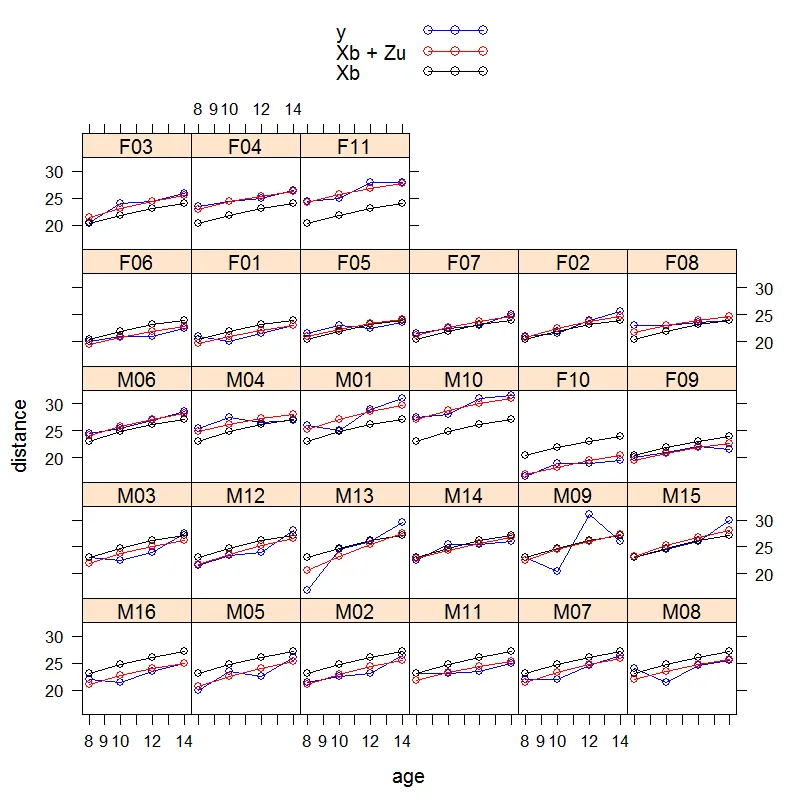
请注意,上图中女性(F##)个体略低于其男性(M##)对应物(黑色线)。例如,在中间区域面板中,M10 <-> F10的差异。
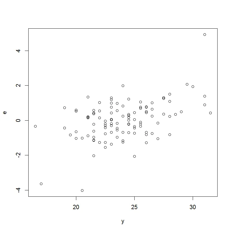
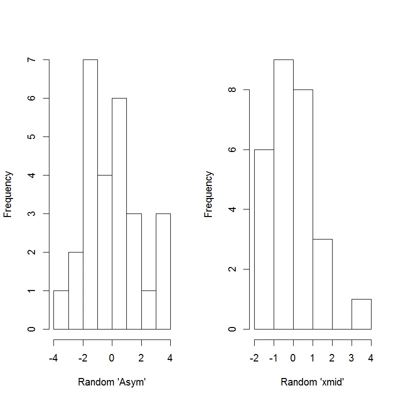
残差和随机效应用于观察指定模型的某些特征。个体M13似乎有点棘手。
 使用lme4软件包,我可以拟合一个非线性混合效应模型,使用逻辑曲线作为我的函数形式。我可以选择将渐近线和中点输入为随机效应。
Error in fn(nM$xeval()) : prss failed to converge in 300 iterations。 - jsta