使用ggplot制作游戏图表

Question

我需要在ggplot中创建一些图形。我可以使用通用的绘图函数来创建它们，但不确定如何在ggplot中实现。以下是我使用常规绘图函数的代码和图表。我正在使用ISLR软件包中的College数据集。

train.2 <- sample(dim(College)[1],2*dim(College)[1]/3)
train.college <- College[train.2,]
test.college <- College[-train.2,]
gam.college <- gam(Outstate~Private+s(Room.Board)+s(Personal)+s(PhD)+s(perc.alumni)+s(Expend)+s(Grad.Rate), data=train.college)
par(mfrow=c(2,2))
plot(gam.college, se=TRUE,col="blue")

- Marvin Bahr

---

请查看 help("plot.gam") 并在 Value 下查找。 - Roland

Answer 1

请看下面更新的答案。

旧答案：

voxel库中有使用ggplot2绘制GAM图的实现。以下是如何进行操作：

library(ISLR)
library(mgcv)
library(voxel)
library(tidyverse)
library(gridExtra)
data(College)

set.seed(1)
train.2 <- sample(dim(College)[1],2*dim(College)[1]/3)
train.college <- College[train.2,]
test.college <- College[-train.2,]
gam.college <- gam(Outstate~Private+s(Room.Board)+s(Personal)+s(PhD)+s(perc.alumni)+s(Expend)+s(Grad.Rate), data=train.college)

vars <- c("Room.Board", "Personal", "PhD", "perc.alumni","Expend", "Grad.Rate")

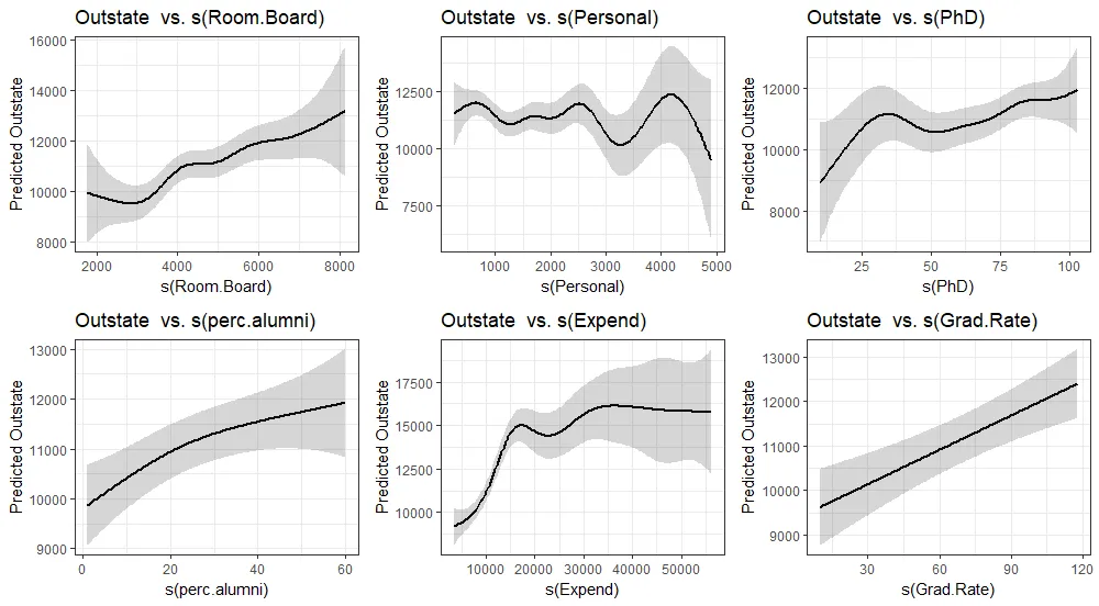
map(vars, function(x){
  p <- plotGAM(gam.college, smooth.cov = x) #plot customization goes here
  g <- ggplotGrob(p)
}) %>%
  {grid.arrange(grobs = (.), ncol = 2, nrow = 3)}

在一连串的错误之后：In plotGAM(gam.college, smooth.cov = x) : 模型拟合中存在一个或多个因子，请考虑按组绘制图形，因为绘图可能不精确

与plot.gam进行比较：

par(mfrow=c(2,3))
plot(gam.college, se=TRUE,col="blue")

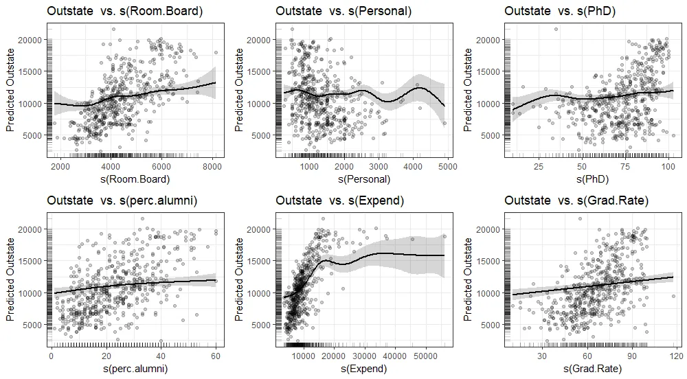
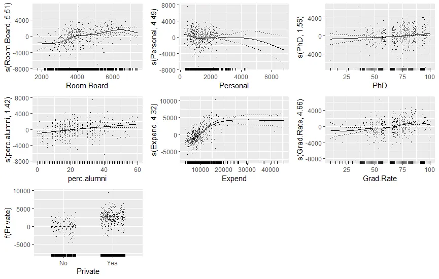
您可能还想绘制观测值：

map(vars, function(x){
  p <- plotGAM(gam.college, smooth.cov = x) +
    geom_point(data = train.college, aes_string(y = "Outstate", x = x ), alpha = 0.2) +
    geom_rug(data = train.college, aes_string(y = "Outstate", x = x ), alpha = 0.2)
  g <- ggplotGrob(p)
}) %>%
  {grid.arrange(grobs = (.), ncol = 3, nrow = 2)}

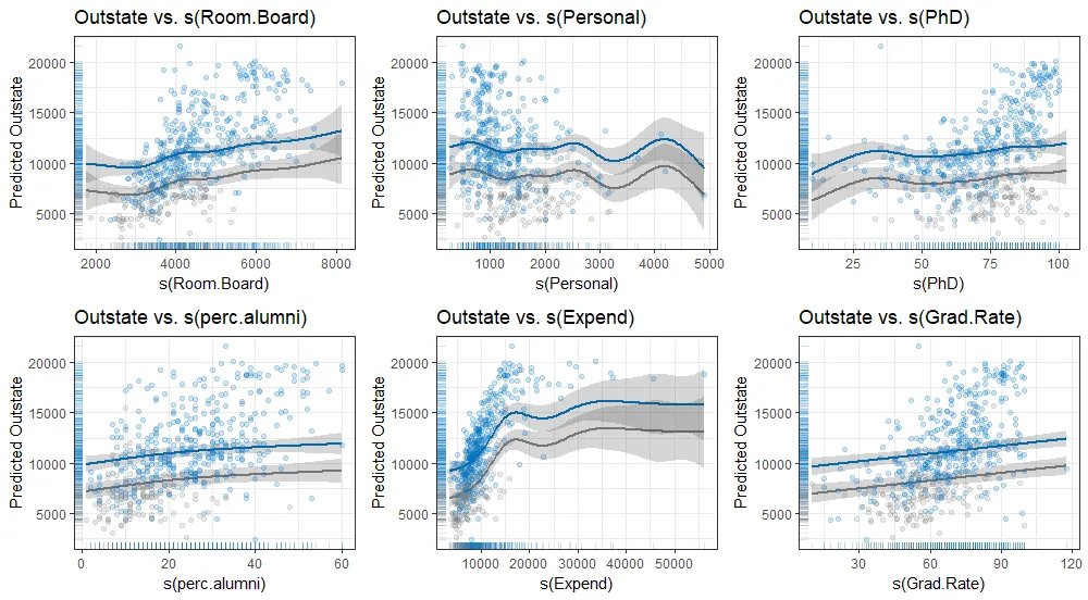
或者按组计算（如果使用了by参数（在gam中为交互作用）则尤其重要。

map(vars, function(x){
  p <- plotGAM(gam.college, smooth.cov = x, groupCovs = "Private") +
    geom_point(data = train.college, aes_string(y = "Outstate", x = x, color= "Private"), alpha = 0.2) +
    geom_rug(data = train.college, aes_string(y = "Outstate", x = x, color= "Private"  ), alpha = 0.2) +
    scale_color_manual("Private", values = c("#868686FF", "#0073C2FF")) +
    theme(legend.position="none")
  g <- ggplotGrob(p)
}) %>%
  {grid.arrange(grobs = (.), ncol = 3, nrow = 2)}

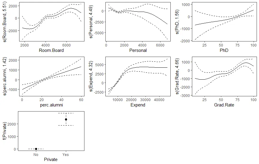
更新，2020年1月8日。

我认为目前包mgcViz提供了比voxel::plotGAM函数更优秀的功能。以下是使用上述数据集和模型的示例：

library(mgcViz)
viz <- getViz(gam.college)
print(plot(viz, allTerms = T), pages = 1)

绘图自定义与ggplot2语法类似：

trt <- plot(viz, allTerms = T) +
  l_points() +
  l_fitLine(linetype = 1)  +
  l_ciLine(linetype = 3) +
  l_ciBar() +
  l_rug() +
  theme_grey() 

print(trt, pages = 1)

这个文档展示了更多的例子。

- missuse

---

在运行该代码后，我遇到了以下错误。plotGAM（gam.college，smooth.cov = x）中的错误：gamFit不是gam类型的对象。 - Marvin Bahr

你正在使用的 gam 方法属于哪个库？如果你能切换到 library(mgcv) 和 mgcv::gam，它可能会起作用。 - missuse

@fibar 是的。生成两个模型，然后生成两个图形，最后使用 gridExtra、cowplot 或其他几个专为此类事情设计的包将它们合并在一个图形中。 - missuse

@误用 我注意到plotGAM和plot的y轴不同。plotGAM中的y轴是因变量的预测值。而plot中的y轴代表什么意思呢？它们的值不相同（例如，8000~16000_与-6000~6000_）。 - T X

有趣的是，现在拟合的GAM模型与使用相同代码发布答案时拟合的模型不同。 - missuse