使用matplotlib / Basemap制作没有河流的世界地图？

Question

是否有办法使用Basemap（或其他方式）绘制大陆的边界，而不必让那些烦人的河流跟着出现？特别是那段连海洋都没到达的刚果河，令人不安。

编辑：我打算在地图上进一步绘制数据，就像Basemap gallery中一样（并且仍然将大陆边界绘制为黑线以便为世界地图提供结构），因此虽然Hooked的解决方案很好，甚至是精湛的，但对于这个目的不适用。

图片由以下产生:

from mpl_toolkits.basemap import Basemap
import matplotlib.pyplot as plt

fig = plt.figure(figsize=(8, 4.5))
plt.subplots_adjust(left=0.02, right=0.98, top=0.98, bottom=0.00)
m = Basemap(projection='robin',lon_0=0,resolution='c')
m.fillcontinents(color='gray',lake_color='white')
m.drawcoastlines()
plt.savefig('world.png',dpi=75)

- Sampo Smolander

---

非常感谢您的赞美！请随意选择最适合您需求的答案（这就是这个网站存在的目的！）。我会保留我的回答，因为它可能对将来的某个人有用。在未来，请确切地说明您想要做什么。我们两个提供的答案都处理了“绘图”部分，我们都将其解释为艺术渲染。但是，您仍然可以在我们提供的答案上绘制图形-所有坐标都在那里，现在您知道所有那些丑陋的河流的位置！ - Hooked

Answer 1

由于这样的原因，我通常完全避免使用 Basemap，而是使用 OGR 读取 shapefile，并将其转换为 Matplotlib artist。 这更费力，但也提供了更多的灵活性。

Basemap 有一些非常不错的功能，比如将输入数据的坐标转换为你的“工作投影”。

如果你想继续使用 Basemap，请获取一个不包含河流的 shapefile。例如，自然地球在物理部分中有一个很好的“陆地”shapefile（下载“比例尺等级”数据并解压缩）。请参阅http://www.naturalearthdata.com/downloads/10m-physical-vectors/

您可以使用 Basemap 的 m.readshapefile() 方法读取 shapefile。这允许您获取投影坐标中的 Matplotlib Path 顶点和代码，然后将其转换为新的 Path。这是一个绕路，但它为您提供了来自 Matplotlib 的所有样式选项，其中大部分直接不可用通过 Basemap。这有点hackish，但我不知道还有其他方法能够基于 Basemap 实现。

所以:

from mpl_toolkits.basemap import Basemap
import matplotlib.pyplot as plt
from matplotlib.collections import PathCollection
from matplotlib.path import Path

fig = plt.figure(figsize=(8, 4.5))
plt.subplots_adjust(left=0.02, right=0.98, top=0.98, bottom=0.00)

# MPL searches for ne_10m_land.shp in the directory 'D:\\ne_10m_land'
m = Basemap(projection='robin',lon_0=0,resolution='c')
shp_info = m.readshapefile('D:\\ne_10m_land', 'scalerank', drawbounds=True)
ax = plt.gca()
ax.cla()

paths = []
for line in shp_info[4]._paths:
    paths.append(Path(line.vertices, codes=line.codes))

coll = PathCollection(paths, linewidths=0, facecolors='grey', zorder=2)

m = Basemap(projection='robin',lon_0=0,resolution='c')
# drawing something seems necessary to 'initiate' the map properly
m.drawcoastlines(color='white', zorder=0)

ax = plt.gca()
ax.add_collection(coll)

plt.savefig('world.png',dpi=75)

给出：

- Rutger Kassies

---

+1 感谢自然地球的参考！您知道其他好的开源软件可以进行“艺术性”渲染吗？ - Hooked

除了Matplotlib，我有时会使用Mapnik（与TileMill一起）。我刚刚注意到我上面的方法忽略/删除了多边形中的内环（例如，里海消失了）:( - Rutger Kassies

非常感谢您迄今为止的帮助，但是我从您提供的链接中下载了ne_10m_land.zip文件，并解压缩后将其读入为'ne_10m_land'，但是我遇到了错误：“line 10, in <module> shp_info = m.readshapefile('ne_10m_land', 'scalerank', drawbounds=True) [...] ValueError: invalid literal for int() with base 10: '****'”。 - Sampo Smolander

我认为这是因为原始的shapefile文件在'scalerank'属性中没有包含有效的整数。输入一些虚拟数字可能会有所帮助。如果没有属性，我不知道Basemap是否可以选择'fid'，这将是很好的。 - Rutger Kassies

你能推荐一个底图替代方案吗？它似乎已被放弃。谢谢。 - tommy.carstensen

请查看Cartopy，它与Matplotlib非常好地集成在一起。详情请见：http://scitools.org.uk/cartopy/docs/latest/gallery.html - Rutger Kassies

Answer 2

如何去除“烦人”的河流：

如果您想要对图像进行后处理（而不是直接使用Basemap），可以删除没有通向海洋的水域：

import pylab as plt
A = plt.imread("world.png")

import numpy as np
import scipy.ndimage as nd
import collections

# Get a counter of the greyscale colors
a      = A[:,:,0]
colors = collections.Counter(a.ravel())
outside_and_water_color, land_color = colors.most_common(2)

# Find the contigous landmass
land_idx = a == land_color[0]

# Index these land masses
L = np.zeros(a.shape,dtype=int) 
L[land_idx] = 1
L,mass_count = nd.measurements.label(L)

# Loop over the land masses and fill the "holes"
# (rivers without outlays)
L2 = np.zeros(a.shape,dtype=int) 
L2[land_idx] = 1
L2 = nd.morphology.binary_fill_holes(L2)

# Remap onto original image
new_land = L2==1
A2 = A.copy()
c = [land_color[0],]*3 + [1,]
A2[new_land] = land_color[0]

# Plot results
plt.subplot(221)
plt.imshow(A)
plt.axis('off')

plt.subplot(222)
plt.axis('off')
B = A.copy()
B[land_idx] = [1,0,0,1]
plt.imshow(B)

plt.subplot(223)
L = L.astype(float)
L[L==0] = None
plt.axis('off')
plt.imshow(L)

plt.subplot(224)
plt.axis('off')
plt.imshow(A2)

plt.tight_layout()  # Only with newer matplotlib
plt.show()

第一张图片是原图，第二张标识了陆地。第三张并不必要，但它可以识别出每个相邻的陆地。第四张图片是你需要的，即去除了“河流”的图片。

- Hooked

---

你的第四张图片仍然有河流。 - tiago

@tiago 是的，但如果您阅读了我的回答，您会注意到所提出的方法是“删除不连接到海洋的水体”，我认为这就是OP所说的“令人烦恼的河流”。做出明确提及的观察并不像提出修复剩余缺陷的建议那样有建设性。 - Hooked

Answer 3

跟随用户1868739的示例，我能够选择我想要的路径（对于某些湖泊）：

from mpl_toolkits.basemap import Basemap
import matplotlib.pyplot as plt

fig = plt.figure(figsize=(8, 4.5))
plt.subplots_adjust(left=0.02, right=0.98, top=0.98, bottom=0.00)
m = Basemap(resolution='c',projection='robin',lon_0=0)
m.fillcontinents(color='white',lake_color='white',zorder=2)
coasts = m.drawcoastlines(zorder=1,color='white',linewidth=0)
coasts_paths = coasts.get_paths()

ipolygons = range(83) + [84] # want Baikal, but not Tanganyika
# 80 = Superior+Michigan+Huron, 81 = Victoria, 82 = Aral, 83 = Tanganyika,
# 84 = Baikal, 85 = Great Bear, 86 = Great Slave, 87 = Nyasa, 88 = Erie
# 89 = Winnipeg, 90 = Ontario
for ipoly in ipolygons:
    r = coasts_paths[ipoly]
    # Convert into lon/lat vertices
    polygon_vertices = [(vertex[0],vertex[1]) for (vertex,code) in
                        r.iter_segments(simplify=False)]
    px = [polygon_vertices[i][0] for i in xrange(len(polygon_vertices))]
    py = [polygon_vertices[i][2] for i in xrange(len(polygon_vertices))]
    m.plot(px,py,linewidth=0.5,zorder=3,color='black')

plt.savefig('world2.png',dpi=100)

但是这仅适用于使用白色背景的大陆。如果我在以下行中将color更改为'gray'，我们会发现其他河流和湖泊没有填充与大陆相同的颜色。(同时调整area_thresh也无法删除连接到海洋的那些河流.)

m.fillcontinents(color='gray',lake_color='white',zorder=2)

这个白色背景的版本足够用于在大陆上进行各种地形信息的进一步彩色绘图，但如果想要保留大陆的灰色背景，则需要更复杂的解决方案。

- Sampo Smolander

---

如果您使用与大陆填充相同的颜色绘制“不需要”的多边形，那么我猜白色河流问题也会消失。 - user1868739

Answer 4

我经常修改Basemap的drawcoastlines()函数，以避免那些“断裂”的河流。为了保持数据源的一致性，我也会修改drawcountries()函数。

以下是我使用的方法，以支持Natural Earth数据中可用的不同分辨率：

from mpl_toolkits.basemap import Basemap


class Basemap(Basemap):
    """ Modify Basemap to use Natural Earth data instead of GSHHG data """
    def drawcoastlines(self):
        shapefile = 'data/naturalearth/coastline/ne_%sm_coastline' % \
                    {'l':110, 'm':50, 'h':10}[self.resolution]
        self.readshapefile(shapefile, 'coastline', linewidth=1.)
    def drawcountries(self):
        shapefile = 'data/naturalearth/countries/ne_%sm_admin_0_countries' % \
                    {'l':110, 'm':50, 'h':10}[self.resolution]
        self.readshapefile(shapefile, 'countries', linewidth=0.5)


m = Basemap(llcrnrlon=-90, llcrnrlat=-40, urcrnrlon=-30, urcrnrlat=+20,
            resolution='l')  # resolution = (l)ow | (m)edium | (h)igh
m.drawcoastlines()
m.drawcountries()

这是输出结果： 请注意，默认情况下Basemap使用分辨率'resolution='c''（粗糙），这在所示代码中不受支持。

- rmolina

---

请注意，要使用此解决方案，您需要从Natural Earth下载数据。 - safay

Answer 5

如果你不介意绘制轮廓而不是shapefiles，那么从任何地方获取海岸线的绘制就非常容易。我从NOAA海岸线提取器中获取了MATLAB格式的海岸线： http://www.ngdc.noaa.gov/mgg/shorelines/shorelines.html 要编辑海岸线，我将其转换为SVG，然后使用Inkscape进行编辑，最后再转换回纬度/经度文本文件（“MATLAB”格式）。

所有Python代码都包含在下面。

# ---------------------------------------------------------------
def plot_lines(mymap, lons, lats, **kwargs) :
    """Plots a custom coastline.  This plots simple lines, not
    ArcInfo-style SHAPE files.

    Args:
        lons: Longitude coordinates for line segments (degrees E)
        lats: Latitude coordinates for line segments (degrees N)

    Type Info:
        len(lons) == len(lats)
        A NaN in lons and lats signifies a new line segment.

    See:
        giss.noaa.drawcoastline_file()
    """

    # Project onto the map
    x, y = mymap(lons, lats)

    # BUG workaround: Basemap projects our NaN's to 1e30.
    x[x==1e30] = np.nan
    y[y==1e30] = np.nan

    # Plot projected line segments.
    mymap.plot(x, y, **kwargs)


# Read "Matlab" format files from NOAA Coastline Extractor.
# See: http://www.ngdc.noaa.gov/mgg/coast/

lineRE=re.compile('(.*?)\s+(.*)')
def read_coastline(fname, take_every=1) :
    nlines = 0
    xdata = array.array('d')
    ydata = array.array('d')
    for line in file(fname) :
#        if (nlines % 10000 == 0) :
#            print 'nlines = %d' % (nlines,)
        if (nlines % take_every == 0 or line[0:3] == 'nan') :
            match = lineRE.match(line)
            lon = float(match.group(1))
            lat = float(match.group(2))

            xdata.append(lon)
            ydata.append(lat)
        nlines = nlines + 1


    return (np.array(xdata),np.array(ydata))

def drawcoastline_file(mymap, fname, **kwargs) :
    """Reads and plots a coastline file.
    See:
        giss.basemap.drawcoastline()
        giss.basemap.read_coastline()
    """

    lons, lats = read_coastline(fname, take_every=1)
    return drawcoastline(mymap, lons, lats, **kwargs)
# =========================================================
# coastline2svg.py
#
import giss.io.noaa
import os
import numpy as np
import sys

svg_header = """<?xml version="1.0" encoding="UTF-8" standalone="no"?>
<!-- Created with Inkscape (http://www.inkscape.org/) -->

<svg
   xmlns:dc="http://purl.org/dc/elements/1.1/"
   xmlns:cc="http://creativecommons.org/ns#"
   xmlns:rdf="http://www.w3.org/1999/02/22-rdf-syntax-ns#"
   xmlns:svg="http://www.w3.org/2000/svg"
   xmlns="http://www.w3.org/2000/svg"
   version="1.1"
   width="360"
   height="180"
   id="svg2">
  <defs
     id="defs4" />
  <metadata
     id="metadata7">
    <rdf:RDF>
      <cc:Work
         rdf:about="">
        <dc:format>image/svg+xml</dc:format>
        <dc:type
           rdf:resource="http://purl.org/dc/dcmitype/StillImage" />
        <dc:title></dc:title>
      </cc:Work>
    </rdf:RDF>
  </metadata>
  <g
     id="layer1">
"""

path_tpl = """
    <path
       d="%PATH%"
       id="%PATH_ID%"
       style="fill:none;stroke:#000000;stroke-width:1px;stroke-linecap:butt;stroke-linejoin:miter;stroke-opacity:1"
"""

svg_footer = "</g></svg>"




# Set up paths
data_root = os.path.join(os.environ['HOME'], 'data')
#modelerc = giss.modele.read_modelerc()
#cmrun = modelerc['CMRUNDIR']
#savedisk = modelerc['SAVEDISK']

ifname = sys.argv[1]
ofname = ifname.replace('.dat', '.svg')

lons, lats = giss.io.noaa.read_coastline(ifname, 1)

out = open(ofname, 'w')
out.write(svg_header)

path_id = 1
points = []
for lon, lat in zip(lons, lats) :
    if np.isnan(lon) or np.isnan(lat) :
        # Process what we have
        if len(points) > 2 :
            out.write('\n<path d="')
            out.write('m %f,%f L' % (points[0][0], points[0][1]))
            for pt in points[1:] :
                out.write(' %f,%f' % pt)
            out.write('"\n   id="path%d"\n' % (path_id))
#            out.write('style="fill:none;stroke:#000000;stroke-width:1px;stroke-linecap:butt;stroke-linejoin:miter;stroke-opacity:1"')
            out.write(' />\n')
            path_id += 1
        points = []
    else :
        lon += 180
        lat = 180 - (lat + 90)
        points.append((lon, lat))


out.write(svg_footer)
out.close()

# =============================================================
# svg2coastline.py

import os
import sys
import re

# Reads the output of Inkscape's "Plain SVG" format, outputs in NOAA MATLAB coastline format

mainRE = re.compile(r'\s*d=".*"')
lineRE = re.compile(r'\s*d="(m|M)\s*(.*?)"')

fname = sys.argv[1]


lons = []
lats = []
for line in open(fname, 'r') :
    # Weed out extraneous lines in the SVG file
    match = mainRE.match(line)
    if match is None :
        continue

    match = lineRE.match(line)

    # Stop if something is wrong
    if match is None :
        sys.stderr.write(line)
        sys.exit(-1)

    type = match.group(1)[0]
    spairs = match.group(2).split(' ')
    x = 0
    y = 0
    for spair in spairs :
        if spair == 'L' :
            type = 'M'
            continue

        (sdelx, sdely) = spair.split(',')
        delx = float(sdelx)
        dely = float(sdely)
        if type == 'm' :
            x += delx
            y += dely
        else :
            x = delx
            y = dely
        lon = x - 180
        lat = 90 - y
        print '%f\t%f' % (lon, lat)
    print 'nan\tnan'

- Bob F

Answer 6

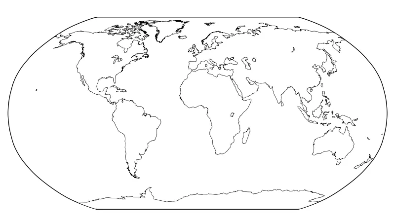
好的，我认为我有一个部分解决方案。

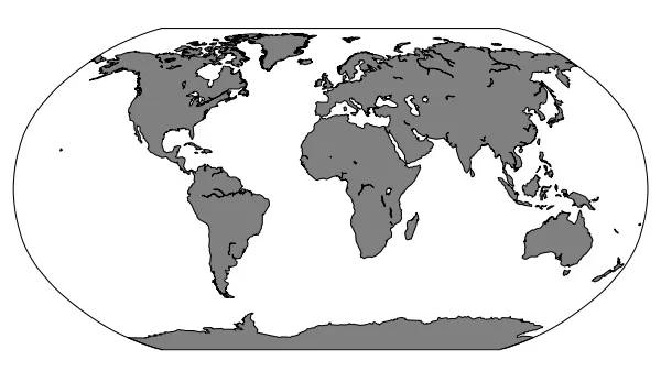
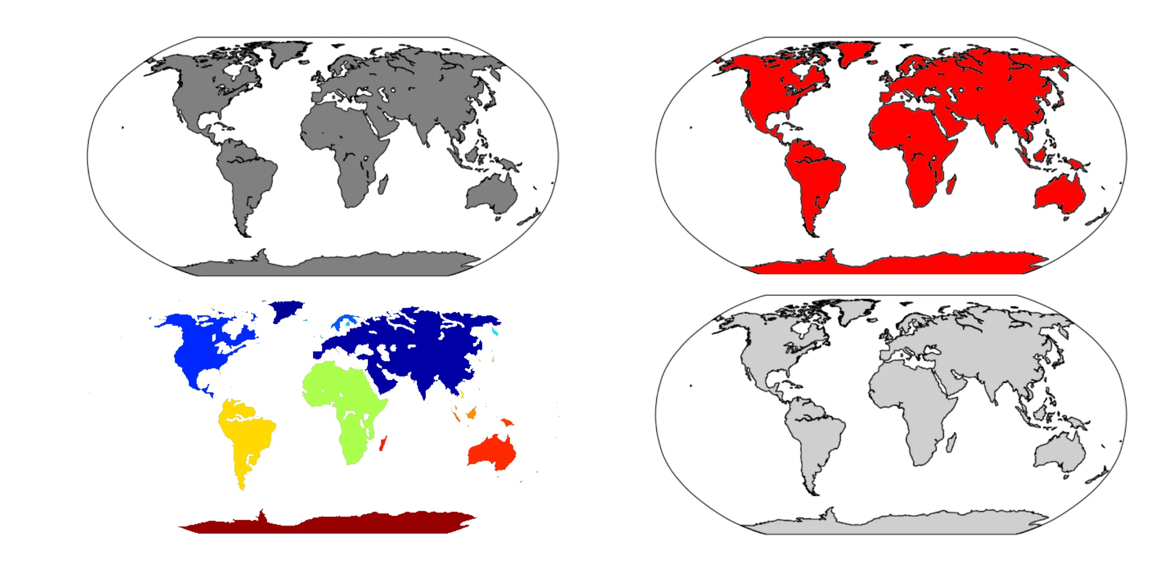
基本的想法是使用 drawcoastlines() 函数中的路径按大小/面积排序。这意味着前 N 条路径（对于大多数应用程序）是主要陆地和湖泊，后面的路径是较小的岛屿和河流。

问题在于，你想要的前 N 条路径将取决于投影方式（例如全球、极地、区域）、是否应用面积阈值以及是否需要湖泊或小岛等。换句话说，你需要根据每个应用程序进行微调。

from mpl_toolkits.basemap import Basemap
import matplotlib.pyplot as plt

mp = 'cyl'
m = Basemap(resolution='c',projection=mp,lon_0=0,area_thresh=200000)

fill_color = '0.9'

# If you don't want lakes set lake_color to fill_color
m.fillcontinents(color=fill_color,lake_color='white')

# Draw the coastlines, with a thin line and same color as the continent fill.
coasts = m.drawcoastlines(zorder=100,color=fill_color,linewidth=0.5)

# Exact the paths from coasts
coasts_paths = coasts.get_paths()

# In order to see which paths you want to retain or discard you'll need to plot them one
# at a time noting those that you want etc. 
for ipoly in xrange(len(coasts_paths)):
    print ipoly
    r = coasts_paths[ipoly]
    # Convert into lon/lat vertices
    polygon_vertices = [(vertex[0],vertex[1]) for (vertex,code) in
                        r.iter_segments(simplify=False)]
    px = [polygon_vertices[i][0] for i in xrange(len(polygon_vertices))]
    py = [polygon_vertices[i][1] for i in xrange(len(polygon_vertices))]
    m.plot(px,py,'k-',linewidth=1)
    plt.show()

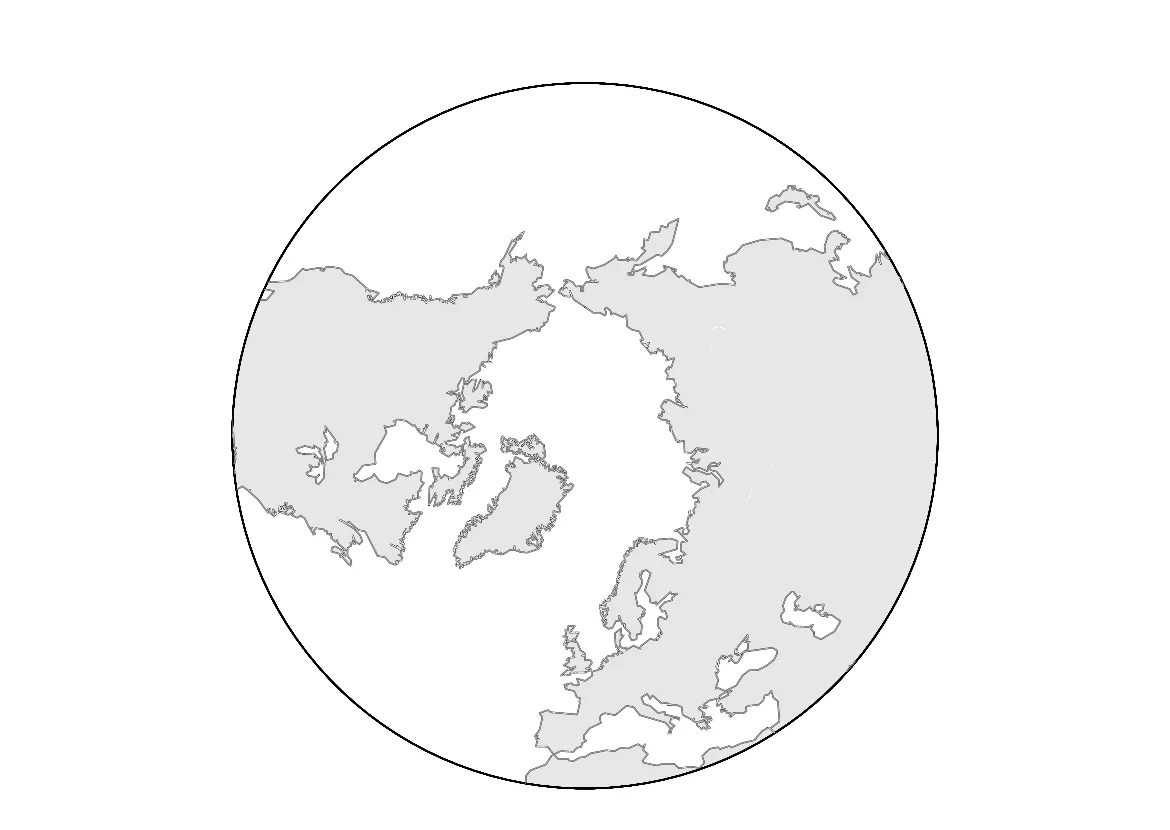
一旦您知道停止绘制的相关ipoly（poly_stop），那么您可以像这样做...

from mpl_toolkits.basemap import Basemap
import matplotlib.pyplot as plt

mproj = ['nplaea','cyl']
mp = mproj[0]

if mp == 'nplaea':
    m = Basemap(resolution='c',projection=mp,lon_0=0,boundinglat=30,area_thresh=200000,round=1)
    poly_stop = 10
else:
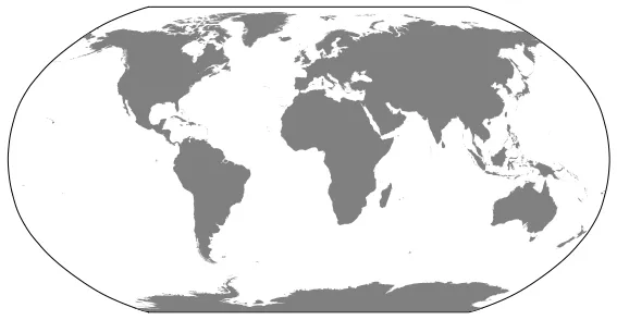
    m = Basemap(resolution='c',projection=mp,lon_0=0,area_thresh=200000)
    poly_stop = 18
fill_color = '0.9'

# If you don't want lakes set lake_color to fill_color
m.fillcontinents(color=fill_color,lake_color='white')

# Draw the coastlines, with a thin line and same color as the continent fill.
coasts = m.drawcoastlines(zorder=100,color=fill_color,linewidth=0.5)

# Exact the paths from coasts
coasts_paths = coasts.get_paths()

# In order to see which paths you want to retain or discard you'll need to plot them one
# at a time noting those that you want etc. 
for ipoly in xrange(len(coasts_paths)):
    if ipoly > poly_stop: continue
    r = coasts_paths[ipoly]
    # Convert into lon/lat vertices
    polygon_vertices = [(vertex[0],vertex[1]) for (vertex,code) in
                        r.iter_segments(simplify=False)]
    px = [polygon_vertices[i][0] for i in xrange(len(polygon_vertices))]
    py = [polygon_vertices[i][1] for i in xrange(len(polygon_vertices))]
    m.plot(px,py,'k-',linewidth=1)
plt.show()

- user1868739

Answer 7

根据我对@sampo-smolander的评论。

from mpl_toolkits.basemap import Basemap
import matplotlib.pyplot as plt

fig = plt.figure(figsize=(8, 4.5))
plt.subplots_adjust(left=0.02, right=0.98, top=0.98, bottom=0.00)
m = Basemap(resolution='c',projection='robin',lon_0=0)
m.fillcontinents(color='gray',lake_color='white',zorder=2)
coasts = m.drawcoastlines(zorder=1,color='white',linewidth=0)
coasts_paths = coasts.get_paths()

ipolygons = range(83) + [84]
for ipoly in xrange(len(coasts_paths)):
    r = coasts_paths[ipoly]
    # Convert into lon/lat vertices
    polygon_vertices = [(vertex[0],vertex[1]) for (vertex,code) in
                        r.iter_segments(simplify=False)]
    px = [polygon_vertices[i][0] for i in xrange(len(polygon_vertices))]
    py = [polygon_vertices[i][1] for i in xrange(len(polygon_vertices))]
    if ipoly in ipolygons:
        m.plot(px,py,linewidth=0.5,zorder=3,color='black')
    else:
        m.plot(px,py,linewidth=0.5,zorder=4,color='grey')
plt.savefig('world2.png',dpi=100)

- user1868739