使用matplotlib在垂直剖面上绘制风向量

Question

我已经搜索过各种资料，但是没有找到关于这个问题的答案。

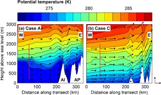
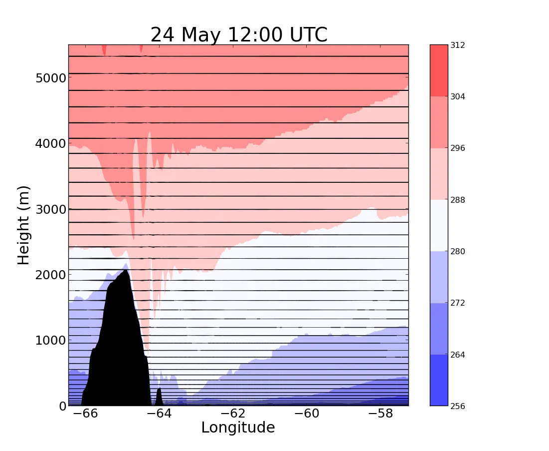
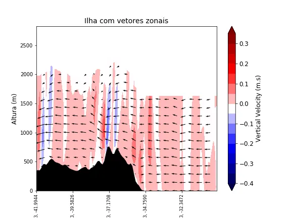
我正在尝试将英国气象局的统一模型在南极半岛上的输出可视化。目前，我有一个经度剖面图，填充轮廓中绘制了潜在温度。我想在其上方绘制风向矢量，使其看起来更像：

我尝试调整matplotlib示例（例如quiver_demo）中给出的纬/经度坐标的示例，但没有成功（可能是因为我做错了一些明显的事情）。

我有风的u、v和w分量（虽然我不需要v，因为我已经从一个纬度线切片中取得了数据）。

我目前正在使用一个名为iris（v1.7）的模块，它允许我处理我拥有的文件（例如将旋转极投影转换为合理的坐标系中的纬度/经度），所以请原谅我的代码中不熟悉的行。

我现在的代码如下：

import iris
import iris.plot as iplt
import matplotlib.pyplot as plt
import numpy as np

# Load variables from file
fname = ['/pathname/filename.pp']
theta= iris.load_cube(fname,'air_potential_temperature') #all data are 3D 'cubes' of dimensions [x,y,z] = [40,800,800]
U = iris.load_cube(fname, 'eastward_wind')
W = iris.load_cube(fname, 'upward_air_velocity')
lev_ht = theta.coord('level_height').points # for extracting z coordinate only - shape = (40,)

##SPATIAL COORDINATES
## rotate projection to account for rotated pole
var_name = theta
pole_lon = 298.5
pole_lat = 22.99
rotated_lat = var_name.coord('grid_latitude').points
rotated_lon = var_name.coord('grid_longitude').points
real_lon, real_lat = iris.analysis.cartography.unrotate_pole(rotated_lon,rotated_lat, pole_lon, pole_lat)

#define function to find index of gridbox in question
def find_gridbox(x,y):
    global lon_index, lat_index
    lat_index = np.argmin((real_lat-x)**2) #take whole array and subtract lat you want from each point, then find the smallest difference
    lon_index = np.argmin((real_lon-y)**2)
    return lon_index, lat_index

lon_index, lat_index = find_gridbox(-66.58333, -63.166667) # coordinates of Cabinet Inlet

#add unrotated lats/lons into variables
lat = var_name.coord('grid_latitude')
lon = var_name.coord('grid_longitude')
New_lat = iris.coords.DimCoord(real_lat, standard_name='latitude',long_name="grid_latitude",var_name="lat",units=lat.units)
New_lon= iris.coords.DimCoord(real_lon, standard_name='longitude',long_name="grid_longitude",var_name="lon",units=lon.units)

var_names = [theta, U, W]

for var in var_names:
    var.remove_coord('grid_latitude')
    var.add_dim_coord(New_lat, data_dim=1)
    var.remove_coord('grid_longitude')
    var.add_dim_coord(New_lon, data_dim=2)

# Create 2D subsets of data for plotting (longitudinal transects)
theta_slice = theta[:,lat_index,:]
U_slice = U[:,lat_index,:]
W_slice = W[:,lat_index,:]

# Create 2d arrays of lon/alt for gridding
x, y = np.meshgrid(lon.points, lev_ht)
u = U_slice
w = W_slice

# plot
fig = plt.figure()
ax1 = fig.add_subplot(111)
ax1.set_axis_bgcolor('k') #set orography to be black
ax3 = iplt.contourf(theta_slice, cmap=plt.cm.bwr)
ax1.set_ylim(0,5500)
barbs = plt.quiver(x, y, u, w)
ax3.set_clim(vmin=250, vmax=320)
ax1.set_title('25 May 00:00 UTC', fontsize=28)
ax1.set_ylabel('Height (m)', fontsize=22)
ax1.set_xlabel('Longitude', fontsize=22)
ax1.tick_params(axis='both', which='major', labelsize=18)
plt.colorbar(ax3)
plt.show()

然而，当向量被绘制时，它们会出现为线条形式：

我不确定这是因为它们太靠近一起了（当我改变线宽和比例等属性时，向量就会非常混乱），还是因为我的输入有误。u和w变量是2D数组（经度/高度），包含风向的西向和上升分量，因此应包含在这些方向上的移动大小。

很抱歉我无法发布实际文件：它们是特定Met Office .pp格式的（当然），但与netCDF具有类似的特性。我已经尝试在代码注释中描述数据维度。

- Shakka

---

我会尝试使用非常简单的barb数据版本——使用zeros_like复制x，y，u，w，然后在中间添加一个箭头，看看是否能够合理绘制。 - cphlewis

@cphlewis - 不错的建议。你说得对，当我这样做时，我遇到了一些非常奇怪的行为，就好像这个向量不知道什么时候结束一样。我将查看数据本身发生了什么，并看是否能够找出我缺失的信息。谢谢。 - Shakka

单位是否可能不匹配？ - cphlewis

@cphlewis 我认为问题在于我需要先计算具有u和v风的向量，然后垂直切割这些数据以正确绘制向量。我正在编写一些代码来解决这个问题，并在获得可行解决方案后发布。 - Shakka

Answer 1

我希望你一切顺利，能够快速解决问题。

下面是一些代码和对应的图像：

import numpy as np
from matplotlib import pyplot
import matplotlib.pyplot as plt
from matplotlib.cm import get_cmap
from matplotlib.colors import from_levels_and_colors
from cartopy import crs
from cartopy.feature import NaturalEarthFeature, COLORS
from netCDF4 import Dataset
from wrf import (getvar, to_np, get_cartopy, latlon_coords, vertcross,
                 cartopy_xlim, cartopy_ylim, interpline, CoordPair)

wrf_file = Dataset("C:/Users/meteorologia.gmmc/Documents/WRF - Rodada Exemplo/wrfout_exemplo.nc")

# Define the cross section start and end points
cross_start = CoordPair(lat=-8.5, lon=-42)
cross_end = CoordPair(lat=-8.5, lon=-30)

# Get the WRF variables
ht = getvar(wrf_file, "z", timeidx=8)
ht = ht[0:20,:,:]
ter = getvar(wrf_file, "ter", timeidx=8)

w = getvar(wrf_file, "wa", timeidx=8)
w = w[0:20,:,:]

u = getvar(wrf_file, "ua", timeidx=8)
u = u[0:20,:,:]

max_dbz = getvar(wrf_file, "mdbz", timeidx=8)

W = 10**(w/10.) # Use linear Z for interpolation

w_cross = vertcross(W, ht, wrfin=wrf_file,
                    start_point=cross_start,
                    end_point=cross_end,
                    latlon=True, meta=True)

U = 10**(u/10.) # Use linear Z for interpolation

u_cross = vertcross(U, ht, wrfin=wrf_file,
                    start_point=cross_start,
                    end_point=cross_end,
                    latlon=True, meta=True)

# Convert back to dBz after interpolation
w_cross = 10.0 * np.log10(w_cross)
u_cross = 10.0 * np.log10(u_cross)

# Add back the attributes that xarray dropped from the operations above
w_cross.attrs.update(w_cross.attrs)
w_cross.attrs["description"] = "destaggered w-wind component"
w_cross.attrs["units"] = "m s-1"

# Add back the attributes that xarray dropped from the operations above
u_cross.attrs.update(u_cross.attrs)
u_cross.attrs["description"] = "destaggered u-wind component"
u_cross.attrs["units"] = "m s-1"

# To remove the slight gap between the dbz contours and terrain due to the
# contouring of gridded data, a new vertical grid spacing, and model grid
# staggering, fill in the lower grid cells with the first non-missing value
# for each column.

# Make a copy of the z cross data. Let's use regular numpy arrays for this.
w_cross_filled = np.ma.copy(to_np(w_cross))
u_cross_filled = np.ma.copy(to_np(u_cross))

# For each cross section column, find the first index with non-missing
# values and copy these to the missing elements below.
for i in range(w_cross_filled.shape[-1]):
    column_vals = w_cross_filled[:,i]
    # Let's find the lowest index that isn't filled. The nonzero function
    # finds all unmasked values greater than 0. Since 0 is a valid value
    # for dBZ, let's change that threshold to be -200 dBZ instead.
    first_idx = int(np.transpose((column_vals > -200).nonzero())[0])
    w_cross_filled[0:first_idx, i] = w_cross_filled[first_idx, i]

# For each cross section column, find the first index with non-missing
# values and copy these to the missing elements below.
for i in range(u_cross_filled.shape[-1]):
    column_vals = u_cross_filled[:,i]
    # Let's find the lowest index that isn't filled. The nonzero function
    # finds all unmasked values greater than 0. Since 0 is a valid value
    # for dBZ, let's change that threshold to be -200 dBZ instead.
    first_idx = int(np.transpose((column_vals > -200).nonzero())[0])
    u_cross_filled[0:first_idx, i] = u_cross_filled[first_idx, i]

# Get the terrain heights along the cross section line
ter_line = interpline(ter, wrfin=wrf_file, start_point=cross_start,
                      end_point=cross_end)

# Get the lat/lon points
lats, lons = latlon_coords(w)

# Get the cartopy projection object
cart_proj = get_cartopy(w)

# Create the figure
fig = pyplot.figure(figsize=(8,6))
ax_cross = pyplot.axes()

# Make the cross section plot for dbz
w_levels = np.arange(-4E-1, +4E-1, 5E-2)
xs = np.arange(0, w_cross.shape[-1], 1)
ys = to_np(w_cross.coords["vertical"])
w_contours = ax_cross.contourf(xs,
                                 ys,
                                 to_np(w_cross_filled),
                                 levels=w_levels,
                                 cmap='seismic',

                                 extend="both")
# Add the color bar
cbar = fig.colorbar(w_contours, ax=ax_cross)
cbar.ax.tick_params(labelsize=12)
cbar.set_label('Vertical Velocity (m.s)', rotation=-270, fontsize=12)
# Fill in the mountain area
ht_fill = ax_cross.fill_between(xs, 0, to_np(ter_line),
                                facecolor="black")

# Tentativa do quiver

ax_cross.quiver(xs[::5], ys[::5],
          to_np(u_cross_filled[::5, ::5]), to_np(w_cross_filled[::5, ::5]*100))

# Set the x-ticks to use latitude and longitude labels
coord_pairs = to_np(u_cross.coords["xy_loc"])
x_ticks = np.arange(coord_pairs.shape[0])
x_labels = [pair.latlon_str() for pair in to_np(coord_pairs)]

# Set the desired number of x ticks below
num_ticks = 5
thin = int((len(x_ticks) / num_ticks) + .5)
ax_cross.set_xticks(x_ticks[::thin])
ax_cross.set_xticklabels(x_labels[::thin], rotation=90, fontsize=8)

# Set the x-axis and  y-axis labels
ax_cross.set_xlabel("Latitude, Longitude", fontsize=12)
ax_cross.set_ylabel("Altura (m)", fontsize=12)

# Add a title
ax_cross.set_title("Ilha com vetores zonais", {"fontsize" : 14})

pyplot.show()

fig.savefig('WV.png', dpi=None, facecolor='w', edgecolor='w',
        orientation='portrait', papertype=None, format=None,
        transparent=False, bbox_inches=None, pad_inches=0.1,
        frameon=None, metadata=None)

- Thiago Luiz

---

非常感谢您提供这段代码。我有一个问题：为什么要将w_cross_filled乘以100？是为了使风的垂直分量（通常被水平风所掩盖）更加明显吗？这样做不会削弱向量的准确性吗？ - BbJug

将 w 乘以 100 只是为了缩放目的，因为其值相对较小（约为 x10-2）。 - Lyndz