ggplot2中的非线性回归线和R²

Question

我有以下数据：

dput(dat)
structure(list(Band = c(1930, 1930, 1930, 1930, 1930, 1930, 1930, 
1930, 1930, 1930, 1930, 1930, 1930, 1930, 1930, 1930, 1930, 1930
), Reflectance = c(25.296494, 21.954657, 18.981184, 15.984661, 
14.381341, 12.485372, 10.592539, 8.51772, 7.601568, 7.075429, 
6.205453, 5.36646, 4.853167, 4.21576, 3.979639, 3.504217, 3.313851, 
2.288752), Number.of.Sprays = c(0, 1, 2, 3, 5, 6, 7, 9, 10, 11, 
14, 17, 19, 21, 27, 30, 36, 49), Legend = structure(c(4L, 1L, 
1L, 1L, 1L, 1L, 1L, 1L, 1L, 1L, 1L, 2L, 2L, 2L, 3L, 3L, 3L, 5L
), .Label = c("1 x spray between each measurement", "2 x spray between each measurement", 
"3 x spray between each measurement", "Dry soil", "Wet soil"), class = "factor")), .Names =c("Band", 
"Reflectance", "Number.of.Sprays", "Legend"), row.names = c(NA, 
-18L), class = "data.frame")

这导致以下图表的生成：

使用以下代码：

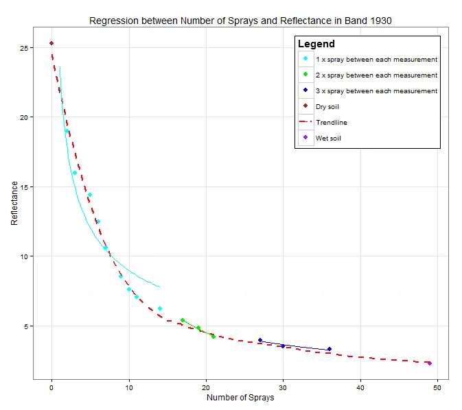
g <- ggplot(dat, aes(Number.of.Sprays, Reflectance, colour = Legend)) +
    geom_point (size = 3) +
    geom_smooth (aes(group = 1, colour = "Trendline"), method = "loess", size = 1, linetype = "dashed", se = FALSE) +
    stat_smooth(method = "nls", formula = "y ~ a*x^b", start = list(a = 1, b = 1), se = FALSE)+
    theme_bw (base_family = "Times") +
    labs (title = "Regression between Number of Sprays and Reflectance in Band 1930") +
    xlab ("Number of Sprays") +
    guides (colour = guide_legend (override.aes = list(linetype = c(rep("blank", 4), "dashed", "blank"), shape = c(rep(16, 4), NA, 16)))) +
    scale_colour_manual (values = c("cyan", "green2", "blue", "brown",  "red", "purple")) +
    theme (legend.title = element_text (size = 15), legend.justification = c(1,1),legend.position = c(1,1), legend.background = element_rect (colour = "black", fill = "white"))

注意：我并不完全理解我的stat_smooth线以及其中的起始特征，只是从另一个帖子中适应过来的。

现在我的问题和目标：

1. 是否有一个包/函数可以提供更准确的估计哪种线性函数最适合点？还是我需要尝试各种功能公式并查看哪个最适合？基于method="loess"的“趋势线”看起来非常好，但我不知道它是如何计算的。

2. 为什么通过stat_smooth()应用的线取决于数据中的因子级别，而不只是依赖于所有数据点？

3. 为什么“趋势线”的虚线图例图标看起来那么糟糕？ (我该怎样改变这个？)

4. 如果我随时有一个适合的非线性回归线，在上面如何计算R²？(summary(lm())只对线性关系进行计算。)是否有可能根据非线性回归线的公式计算R²？

我知道这是很多问题，也许其中一些与统计学相关而不是直接与R相关。如果有什么不对，请编辑这个问题。

感谢您的所有帮助， Patrick

- pat-s

---

1. 你传递给 nls 的函数应该基于数据背后的科学选择。loess 是一个平滑器，即非参数拟合。
2. 因为你映射了 colour = Legend。
3. 你所说的“坏”是什么意思？
4. https://stat.ethz.ch/pipermail/r-help/2002-July/023461.html

- Roland

1. 好的，所以没有可以为我完成这个任务的“函数”或工具？例如，对于Excel，您可以使用http://www.nutonian.com/products/eureqa/。
2. 那很有道理。如果我把它删除，我的代码就不能正常工作了，我会收到一个奇怪的错误消息 =/
3. 我的意思是图标看起来厚度不一致，有一条粗线和小点。更希望/期望作为符号的是2个相等的破折号？
4. 谢谢！

- pat-s

我的意思是你不应该使用这样的工具。 - Roland

Answer 1

1) 也许我误解了问题，但我认为您要求的是一种理性和半自动的方法来估计NLS方法的最佳起始点，因为loess方法不提供您可以在未来使用的模型表达式。

如果是这种情况，那么我来了。在您的方程中，a需要相对接近于Number of Sprays = 0时Reflectance的期望值，而b应该给出Reflectance随着Number of Sprays下降的想法，以便高斯-牛顿算法能够很好地完成其工作。 a和b的值不需要太准确。您可以尝试以下内容：

fit = lm ( data = dat, Reflectance ~ Number.of.Sprays )

然后，在您的ggplot调用中，我会将您的geom_smooth语句替换为：

stat_smooth(method = "nls", formula = "y ~ a*x^b",  method.args = list(start=c(a=fit$coefficients[[1]], b=fit$coefficients[[2]])), se = FALSE)

关于NLS法的起始值的警告将消失，它会很好地收敛。

4）作为拟合优度的一个指标，我建议你计算观测值和预测值之间的相关性。注意，当包括截距时，R2仅是观测结果和观测预测变量值之间样本相关系数的平方。所以这对你应该有用：

r2 =  cor (dat$Reflectance, predict(fit))^2

2,3) 关于这些小问题，我无法给出直接的答案，或者我没有很好地理解它们。当您将Legend用作美学元素时，您绘制的线条是基于因子水平而不是其他情况。

- elcortegano