我基本上完全按照 @jwimberley 的想法,并想在这里分享我的结果。 我创建了一个类,它执行以下操作:
- 构造函数参数:
- CDF(归一化或非归一化),它是PDF的积分。
- 分布的下限和上限
- (可选)决定我们应该取多少CDF样本点的分辨率。
- 计算从CDF -> 随机数 x的映射。这是我们的反向CDF函数。
- 通过以下方式生成随机点:
- 使用
std::random生成介于(0, 1]之间的随机概率p。
- 在我们的映射中进行二分查找,找到与p对应的CDF值。返回与CDF一起计算的x。提供附近“桶”之间的可选线性插值,否则我们将得到n == 分辨率离散步骤。
代码:
#ifndef SAMPLED_DISTRIBUTION
#define SAMPLED_DISTRIBUTION
#include <algorithm>
#include <vector>
#include <random>
#include <stdexcept>
template <typename T = double, bool Interpolate = true>
class Sampled_distribution
{
public:
using CDFFunc = T (*)(T);
Sampled_distribution(CDFFunc cdfFunc, T low, T high, unsigned resolution = 200)
: mLow(low), mHigh(high), mRes(resolution), mDist(0.0, 1.0)
{
if (mLow >= mHigh) throw InvalidBounds();
mSampledCDF.resize(mRes + 1);
const T cdfLow = cdfFunc(low);
const T cdfHigh = cdfFunc(high);
T last_p = 0;
for (unsigned i = 0; i < mSampledCDF.size(); ++i) {
const T x = i/mRes*(mHigh - mLow) + mLow;
const T p = (cdfFunc(x) - cdfLow)/(cdfHigh - cdfLow);
if (! (p >= last_p)) throw CDFNotMonotonic();
mSampledCDF[i] = Sample{p, x};
last_p = p;
}
}
template <typename Generator>
T operator()(Generator& g)
{
T cdf = mDist(g);
auto s = std::upper_bound(mSampledCDF.begin(), mSampledCDF.end(), cdf);
auto bs = s - 1;
if (Interpolate && bs >= mSampledCDF.begin()) {
const T r = (cdf - bs->prob)/(s->prob - bs->prob);
return r*bs->value + (1 - r)*s->value;
}
return s->value;
}
private:
struct InvalidBounds : public std::runtime_error { InvalidBounds() : std::runtime_error("") {} };
struct CDFNotMonotonic : public std::runtime_error { CDFNotMonotonic() : std::runtime_error("") {} };
const T mLow, mHigh;
const double mRes;
struct Sample {
T prob, value;
friend bool operator<(T p, const Sample& s) { return p < s.prob; }
};
std::vector<Sample> mSampledCDF;
std::uniform_real_distribution<> mDist;
};
#endif
以下是翻译的结果:
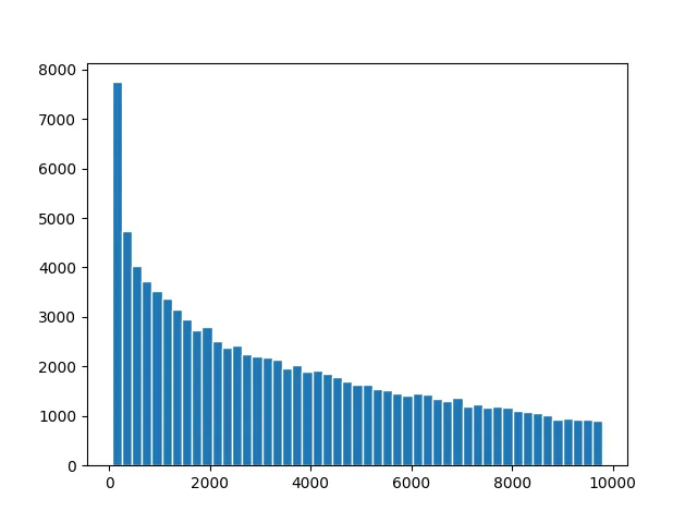
这里是一些结果的图表。对于给定的概率密度函数,我们需要首先通过积分来解析计算累积分布函数。
对数线性
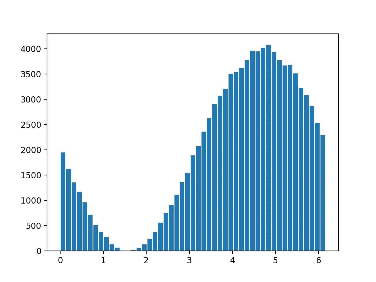
正弦波形
您可以使用以下演示来尝试:
#include "sampled_distribution.hh"
#include <iostream>
#include <fstream>
int main()
{
auto logFunc = [](double x) {
const double k = -1.0;
const double m = 10;
return x*(k*std::log(x) + m - k);
};
auto sinFunc = [](double x) { return x + std::cos(x); };
std::mt19937 gen;
Sampled_distribution<> dist(sinFunc, 0.0, 6.28);
std::ofstream file("d.txt");
for (int i = 0; i < 100000; i++) file << dist(gen) << std::endl;
}
数据是用Python绘制的。
import numpy as np
import matplotlib.pyplot as plt
d = np.loadtxt("d.txt")
fig, ax = plt.subplots()
bins = np.arange(d.min(), d.max(), (d.max() - d.min())/50)
ax.hist(d, edgecolor='white', bins=bins)
plt.show()
使用以下命令运行演示:
clang++ -std=c++11 -stdlib=libc++ main.cc -o main; ./main; python dist_plot.py
m和k的预期范围以及范围。特别地,是否考虑x小于1? - Walter