在R中决定glm逻辑回归模型的阈值

Question

我有一些带有预测变量和二元目标的数据。例如：

df <- data.frame(a=sort(sample(1:100,30)), b= sort(sample(1:100,30)), 
                 target=c(rep(0,11),rep(1,4),rep(0,4),rep(1,11)))

我使用glm()训练了一个逻辑回归模型。

model1 <- glm(formula= target ~ a + b, data=df, family=binomial)

现在我正在尝试预测输出结果（对于这个示例，相同的数据应该足够）

predict(model1, newdata=df, type="response")

这将生成一组概率数字向量。但是我想预测实际的类别。我可以在概率数字上使用round()函数，但这假设任何低于0.5的都是类别“0”，而任何高于此值的都是类别“1”。这是正确的假设吗？即使每个类别的人口可能不相等（或接近相等）？还是有一种方法来估算这个阈值？

- user2175594

---

有不同的标准，例如灵敏度和特异性之和最大的点，可以参考这个问题：https://dev59.com/E37aa4cB1Zd3GeqPvNEK#23133261 - adibender

@adibender 谢谢！但是把阈值作为人口比例肯定是不正确的，对吧？也就是说，如果在人口中，30% 的情况是 '0'，而 70% 是 '1'，那么一个天真的估计是使用 0.3 作为阈值。但这不是一个逻辑上正确的方法来处理这个问题，对吗？ - user2175594

你可以在这里找到一个关于该主题的很棒的教程：https://hopstat.wordpress.com/2014/12/19/a-small-introduction-to-the-rocr-package/ - pbahr

Answer 1

在glm模型中，最好的阈值（或截断点）是使特异性和灵敏度最大化的点。该阈值可能不会在您的模型中给出最高的预测，但它不会偏向于阳性或阴性。ROCR包含可以帮助您执行此操作的函数。请查看此包中的performance()函数。它将为您提供所需结果。以下是您期望获得的图片：

找到截断点后，我通常编写自己的函数来查找其预测值高于截断值的数据点数量，并将其与所属的组匹配。

- Error404

---

能否提供一个生成上述图形的更具体的代码？另外，当概率值介于0和1之间时，如何将截止值设置在0至14之间？ - Kasia Kulma

我在下面添加了baseR/ggplot方法！ - user61871

Answer 2

确定好的模型参数，包括逻辑回归中“我应该设置什么阈值”，最好的方法是使用交叉验证。

一般的想法是保留训练集的一个或多个部分，并选择在这个保留的集合上正确分类数量最大的阈值，但是维基百科可以给你更多详细信息。

- merlin2011

---

由于我们将在交叉验证数据上调整阈值参数，因此，这需要一个第三个保留集来评估并报告无偏的预期误差？ - user2175594

@user2175594，是的，那是正確的。傳統上，你至少需要三個獨立的數據分區：訓練、驗證和測試（評估）。但是，如果你正在進行像 k-fold 交叉驗證這樣的操作，那麼訓練和驗證本質上是同一組數據，在多種方式下重新分區。 - merlin2011

Answer 3

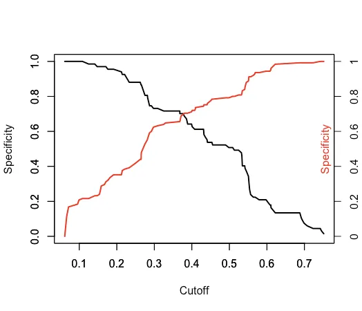
在尝试复制第一个图表时四处使用工具。给定一个 predictions <- prediction(pred,labels) 对象，然后使用基础R方法。

plot(unlist(performance(predictions, "sens")@x.values), unlist(performance(predictions, "sens")@y.values), 
     type="l", lwd=2, ylab="Specificity", xlab="Cutoff")
par(new=TRUE)
plot(unlist(performance(predictions, "spec")@x.values), unlist(performance(predictions, "spec")@y.values), 
     type="l", lwd=2, col='red', ylab="", xlab="")
axis(4, at=seq(0,1,0.2),labels=z)
mtext("Specificity",side=4, padj=-2, col='red')

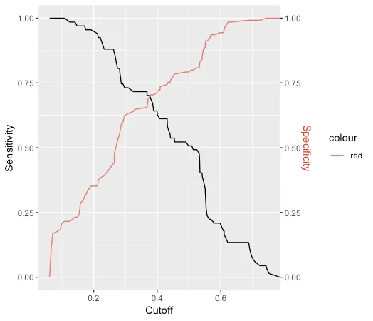
"ggplot2方法

"

sens <- data.frame(x=unlist(performance(predictions, "sens")@x.values), 
                   y=unlist(performance(predictions, "sens")@y.values))
spec <- data.frame(x=unlist(performance(predictions, "spec")@x.values), 
                   y=unlist(performance(predictions, "spec")@y.values))

sens %>% ggplot(aes(x,y)) + 
  geom_line() + 
  geom_line(data=spec, aes(x,y,col="red")) +
  scale_y_continuous(sec.axis = sec_axis(~., name = "Specificity")) +
  labs(x='Cutoff', y="Sensitivity") +
  theme(axis.title.y.right = element_text(colour = "red"), legend.position="none") 

- user61871

Answer 4

为了在具有最接近敏感性和特异性值的数据中获得阈值（即上面的图表中的交叉点），您可以使用以下代码进行编程，这将非常接近：

要以程序方式获取此阈值，请使用以下代码：

predictions = prediction(PREDS, LABELS)

sens = cbind(unlist(performance(predictions, "sens")@x.values), unlist(performance(predictions, "sens")@y.values))
spec = cbind(unlist(performance(predictions, "spec")@x.values), unlist(performance(predictions, "spec")@y.values))
sens[which.min(apply(sens, 1, function(x) min(colSums(abs(t(spec) - x))))), 1]

- Adam Waring

Answer 5

函数PresenceAbsence::optimal.thresholds在PresenceAbsence包中实现了12种方法。

这也在Freeman, E. A., & Moisen, G. G. (2008)的论文《A comparison of the performance of threshold criteria for binary classification in terms of predicted prevalence and kappa》中有所涉及，该论文探讨了二元分类的阈值准则在预测普遍性和kappa方面的表现比较。

- irudnyts

Answer 6

你可以尝试以下方法：

perfspec <- performance(prediction.obj = pred, measure="spec", x.measure="cutoff")

plot(perfspec)

par(new=TRUE)

perfsens <- performance(prediction.obj = pred, measure="sens", x.measure="cutoff")

plot(perfsens)

- Dipayan Sarkar