使用matplotlib实现半球坐标的平滑2D绘图

4

我有一些位于半球上的点(theta在0到90的范围内,phi在0到180的范围内)。我希望绘制一个二维热图,因为三维图形会产生遮挡。此外,由于n个点位于间隔均匀的位置,平滑的图形(例如高斯平滑)可能看起来更好。

我的尝试:我在matplotlib的这里找到了一个极坐标图,它看起来有点像我想要的,但是(a)网格坐标标错了,(b)没有对间隔点进行平滑处理。

编辑:我的最小工作示例

import numpy as np
import matplotlib.pyplot as plt

def to_degrees(x):
    return x*np.pi/180.0

def get_projection(phi, lmda, phi_0=0.0, lmda_0=to_degrees(90.0)):
    # Credits : https://en.wikipedia.org/wiki/Orthographic_map_projection
    x = np.cos(phi)*np.sin(lmda - lmda_0)
    y = np.cos(phi_0)*np.sin(phi) - np.sin(phi_0)*np.cos(phi)*np.cos(lmda-lmda_0)
    return [x, y]

# Adding latitudes and longitudes to give the appearance of a sphere
latitudes = [60, 30, 0, -30, -60] #elevations
longitudes = [0, 30, 60, 90, 120, 150, 180] #azimuths

plt.gca().set_aspect('equal', adjustable='box')
for longitude in longitudes:
    prev_point = get_projection(to_degrees(-90.), to_degrees(0))
    for latitude in range(-90, 90):
        curr_point = get_projection(to_degrees(latitude), to_degrees(longitude))
        plt.plot([prev_point[0], curr_point[0]], [prev_point[1], curr_point[1]], 'k', alpha=0.3)
        prev_point = curr_point

for latitude in latitudes:
    prev_point = get_projection(to_degrees(latitude), to_degrees(0))
    for longitude in range(0, 180):
        curr_point = get_projection(to_degrees(latitude), to_degrees(longitude))
        plt.plot([prev_point[0], curr_point[0]], [prev_point[1], curr_point[1]], 'k', alpha=0.3)
        prev_point = curr_point

views = [[-60, 0], [60, 0]] # and similar points of the format [azimuth, elevation]
frequency = [0.5, 0.3] # and similar numbers in range [0,1] for heatmap

for view_idx in range(len(views)):
    loc = get_projection(to_degrees(views[view_idx][0]), to_degrees(views[view_idx][1]))
    plt.scatter(loc[0], loc[1], s=300, c=np.array(plt.cm.jet(frequency[view_idx])).reshape(1, -1))

plt.show()

获得这个

在此输入图片描述

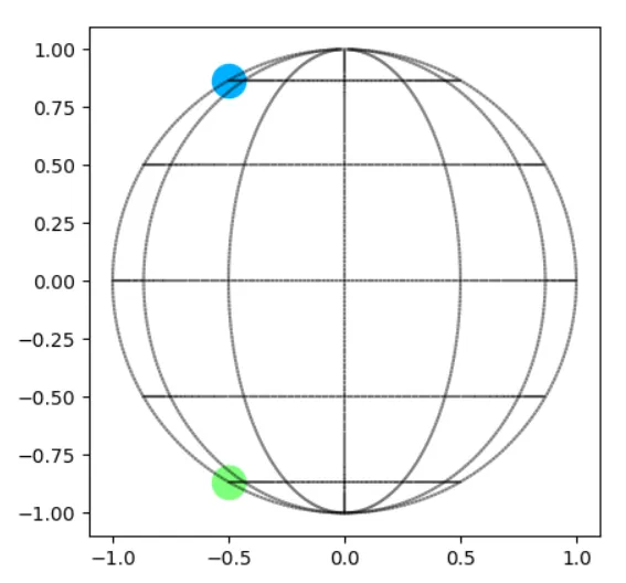
由于我有11-12个这样的点分布在整个半球上,我希望使热图变得更加平滑。
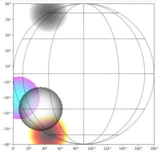

2
你需要提供一个最小、完整和可验证的示例,其中包括一个玩具数据集(参考如何创建良好的可重现的pandas示例)。 - Diziet Asahi
1
正如@DizietAsahi所说,请提供一个我们可以使用的示例。除此之外,例如这个答案,在极坐标下绘制griddatapcolormesh是否与您想要的视觉效果接近? - Asmus
谢谢,我的尝试看起来有些相似,但现在我想要平滑散点图。仅对一个有限的圆进行平滑处理有些具有挑战性,其他在SO上的答案似乎无法解决这个问题。 - thechargedneutron
1个回答

1

根据这篇文章

您可以创建一个网格,使用函数计算颜色,然后使用插值imshow

我编写了一个名为create_gaussian_mesh的函数来解决问题

def create_gaussian_mesh(views,cmap_names,t_x,t_y,radii,ax):
    """
    views: the points
    cmap_names: for heatmap
    t_x: the number of grids in x direction 
    t_y: the number of grids in y direction 
    radii: the radii of the Gaussians to plot
    ax: the canvas 
    """
    def gaussian(view,radius):
        
        # initialize a patch and grids  
        patch = np.empty((t_x,t_y))
        patch[:,:] = np.nan
        x = np.linspace(-1,1,t_x)
        y = np.linspace(-1,1,t_y)
        x_grid,y_grid = np.meshgrid(x, y)
    
        loc = get_projection(to_degrees(view[0]),to_degrees(view[1]))
        # threshold controls the size of the gaussian 
        circle_mask = (x_grid-loc[0])**2 + (y_grid-loc[1])**2 < radius
        gaussian_value = np.exp((x_grid-loc[0])**2+(y_grid-loc[1])**2)
        patch[circle_mask] = gaussian_value[circle_mask]
    
        return patch

    # modify the patch
    for view,cmap_name,radius in zip(views,cmap_names,radii): 
        patch = gaussian(view,radius)
        extent = -1,1,-1,1
        cmap = plt.get_cmap(cmap_name)
        ax.imshow(patch,cmap=cmap,alpha=.6,interpolation='bilinear',extent=extent)

使用此函数,您可以绘制您的数据。
import numpy as np
import matplotlib.pyplot as plt

to_degrees = lambda x: np.deg2rad(x)

def get_projection(phi, lmda, phi_0=0.0, lmda_0=to_degrees(90.0)):
    # Credits : https://en.wikipedia.org/wiki/Orthographic_map_projection
    x = np.cos(phi)*np.sin(lmda - lmda_0)
    y = np.cos(phi_0)*np.sin(phi) - np.sin(phi_0)*np.cos(phi)*np.cos(lmda-lmda_0)
    return x, y

# Adding latitudes and longitudes to give the appearance of a sphere
latitudes = [60, 30, 0, -30, -60] #elevations
longitudes = [0, 30, 60, 90, 120, 150, 180] #azimuths

fig,ax = plt.subplots(figsize=(8,8))
ax.set_aspect('equal', adjustable='box')
ax.set_xlim(-1,1)
ax.set_ylim(-1,1)
# set the right ticks 
x_ticks = ['$%i\degree$' % ind for ind in np.linspace(0,180,10).astype(int)]
y_ticks = ['$%i\degree$' % ind for ind in np.linspace(-90,90,10).astype(int)]
ax.set_xticks(np.linspace(-1,1,10));ax.set_xticklabels(x_ticks)
ax.set_yticks(np.linspace(-1,1,10));ax.set_yticklabels(y_ticks)

for longitude in longitudes:
    prev_point = get_projection(to_degrees(-90.), to_degrees(0))
    for latitude in range(-90, 90):
        curr_point = get_projection(to_degrees(latitude), to_degrees(longitude))
        ax.plot([prev_point[0], curr_point[0]], [prev_point[1], curr_point[1]], 'k', alpha=0.3)
        prev_point = curr_point
for latitude in latitudes:
    prev_point = get_projection(to_degrees(latitude), to_degrees(0))
    for longitude in range(0, 180):
        curr_point = get_projection(to_degrees(latitude), to_degrees(longitude))
        ax.plot([prev_point[0], curr_point[0]], [prev_point[1], curr_point[1]], 'k', alpha=0.3)
        prev_point = curr_point

views = [[-60, 0], [60, 0], [20,10],[30,45]] # and similar points of the format [azimuth, elevation]
# instead of frequencies, you need a list of names of cmaps 
cmap_names= ['gray','hot','cool','Greys']
    
# the radius of the gaussians to plot 
radii = np.linspace(0.08,0.1,len(views))
create_gaussian_mesh(views,cmap_names,t_x=300,t_y=300,radii=radii,ax=ax)

其中x和y轴的刻度已经正确设置。代码的输出图如下:

output


网页内容由stack overflow 提供, 点击上面的
可以查看英文原文,
原文链接