开放量子系统建模

Question

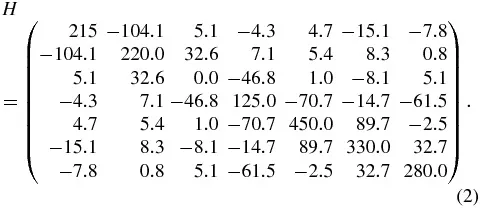
我已经长时间在使用Lindblad Equation对开放量子系统建模。哈密顿量如下：

然而，另外两个矩阵被添加到哈密顿量中。其中一个矩阵的所有对角线项均为-33.3333i，其余为零。另一个矩阵的第三个对角线项等于-0.033333i。

林德布拉德方程如下：

其中L_i是矩阵（列表中的[L1，L2，L3，L4，L5，L6，L7]）。 L_i的矩阵只是一个7x7矩阵，除了L_(ii)=1之外，所有元素都为零。 H是总哈密顿量，是密度矩阵，是常数，等于，其中T是温度，k是玻尔兹曼常数，，其中h是普朗克常数。（请注意，gamma在natural units中）

以下代码解决了林德布拉德方程，从而计算出密度矩阵。然后它计算并绘制了随时间变化的密度矩阵：

这被称为站点3种群。 被称为 bra（布拉）, 被称为 ket（凯特）。它们都是向量。在本例中，请查看它们的定义代码。

以下是代码：

from qutip import Qobj, Options, mesolve
import numpy as np
import scipy
from math import *
import matplotlib.pyplot as plt

hamiltonian = np.array([
    [215, -104.1, 5.1, -4.3, 4.7, -15.1, -7.8],
    [-104.1, 220.0, 32.6, 7.1, 5.4, 8.3, 0.8],
    [5.1, 32.6, 0.0, -46.8, 1.0, -8.1, 5.1],
    [-4.3, 7.1, -46.8, 125.0, -70.7, -14.7, -61.5],
    [4.7, 5.4, 1.0, -70.7, 450.0, 89.7, -2.5],
    [-15.1, 8.3, -8.1, -14.7, 89.7, 330.0, 32.7],
    [-7.8, 0.8, 5.1, -61.5, -2.5, 32.7, 280.0]
])

recomb = np.zeros((7, 7), dtype=complex)
np.fill_diagonal(recomb, 33.33333333)
recomb = recomb * -1j
trap = np.zeros((7, 7), complex)
trap[2][2] = -0.033333333333j
hamiltonian = recomb + trap + hamiltonian
H = Qobj(hamiltonian)

# Note the extra .0 on the end to convert to float
gamma = (2 * pi) * (296 * 0.695) * (35.0 / 150)

L1 = np.array([
    [1, 0, 0, 0, 0, 0, 0], [0, 0, 0, 0, 0, 0, 0],
    [0, 0, 0, 0, 0, 0, 0], [0, 0, 0, 0, 0, 0, 0],
    [0, 0, 0, 0, 0, 0, 0], [0, 0, 0, 0, 0, 0, 0],
    [0, 0, 0, 0, 0, 0, 0]
])

L2 = np.array([
    [0, 0, 0, 0, 0, 0, 0], [0, 1, 0, 0, 0, 0, 0],
    [0, 0, 0, 0, 0, 0, 0], [0, 0, 0, 0, 0, 0, 0],
    [0, 0, 0, 0, 0, 0, 0], [0, 0, 0, 0, 0, 0, 0],
    [0, 0, 0, 0, 0, 0, 0]
])

L3 = np.array([
    [0, 0, 0, 0, 0, 0, 0], [0, 0, 0, 0, 0, 0, 0],
    [0, 0, 1, 0, 0, 0, 0], [0, 0, 0, 0, 0, 0, 0],
    [0, 0, 0, 0, 0, 0, 0], [0, 0, 0, 0, 0, 0, 0],
    [0, 0, 0, 0, 0, 0, 0]
])      

L4 = np.array([
    [0, 0, 0, 0, 0, 0, 0], [0, 0, 0, 0, 0, 0, 0],
    [0, 0, 0, 0, 0, 0, 0], [0, 0, 0, 1, 0, 0, 0],
    [0, 0, 0, 0, 0, 0, 0], [0, 0, 0, 0, 0, 0, 0],
    [0, 0, 0, 0, 0, 0, 0]
])

L5 = np.array([
    [0, 0, 0, 0, 0, 0, 0], [0, 0, 0, 0, 0, 0, 0],
    [0, 0, 0, 0, 0, 0, 0], [0, 0, 0, 0, 0, 0, 0],
    [0, 0, 0, 0, 1, 0, 0], [0, 0, 0, 0, 0, 0, 0],
    [0, 0, 0, 0, 0, 0, 0]
])

L6 = np.array([
    [0, 0, 0, 0, 0, 0, 0], [0, 0, 0, 0, 0, 0, 0],
    [0, 0, 0, 0, 0, 0, 0], [0, 0, 0, 0, 0, 0, 0],
    [0, 0, 0, 0, 0, 0, 0], [0, 0, 0, 0, 0, 1, 0],
    [0, 0, 0, 0, 0, 0, 0]
])

L7 = np.array([
    [0, 0, 0, 0, 0, 0, 0], [0, 0, 0, 0, 0, 0, 0],
    [0, 0, 0, 0, 0, 0, 0], [0, 0, 0, 0, 0, 0, 0],
    [0, 0, 0, 0, 0, 0, 0], [0, 0, 0, 0, 0, 0, 0],
    [0, 0, 0, 0, 0, 0, 1]
])

# Since our gamma variable cannot be directly applied onto
# the Lindblad operator, we must multiply it with
# the collapse operators:  

rho0=Qobj(L1)

L1 = Qobj(gamma * L1)
L2 = Qobj(gamma * L2)
L3 = Qobj(gamma * L3)
L4 = Qobj(gamma * L4)
L5 = Qobj(gamma * L5)
L6 = Qobj(gamma * L6)
L7 = Qobj(gamma * L7)

options = Options(nsteps=1000000, atol=1e-5)

bra3 = [[0, 0, 1, 0, 0, 0, 0]]
bra3q = Qobj(bra3)

ket3 = [[0], [0], [1], [0], [0], [0], [0]]
ket3q = Qobj(ket3)

starttime = 0
# this is effectively just a label - `mesolve` alwasys starts from `rho0` -
# it's just saying what we're going to call the time at t0
endtime = 100
# Arbitrary - this solves with the options above
# (max 1 million iterations to converge - tolerance 1e-10)
num_intermediate_state = 100

state_evaluation_times = np.linspace(
    starttime,
    endtime,
    num_intermediate_state
)

result = mesolve(
    H,
    rho0,
    state_evaluation_times,
    [L1, L2, L3, L4, L5, L6, L7],
    [],
    options=options
)

number_of_interest = bra3q * (result.states * ket3q)

points_to_plot = []
for number in number_of_interest:
    if number == number_of_interest[0]:
        points_to_plot.append(0)
    else:
        points_to_plot.append(number.data.data.real[0])

plt.plot(state_evaluation_times, points_to_plot)
plt.show()
exit()

这段代码使用了一个名为qutip的Python模块。它内置了一个Lindblad方程求解器，使用scipy.integrate.odeint。

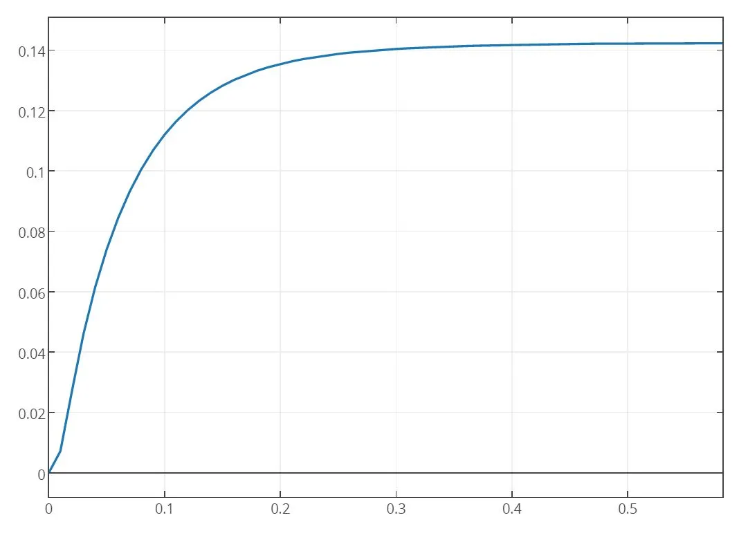
目前，该程序显示如下：

然而，网站3的人口极限应该为0。因此，它应该慢慢降低到零。特别是在t=75时，下降应该开始。

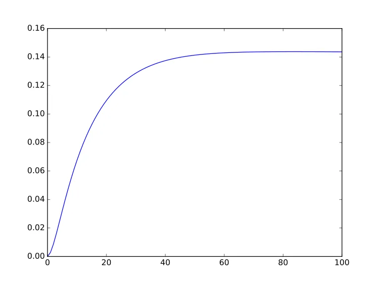
这段代码可以运行，但并没有产生我所解释的正确结果。那么，为什么它没有产生正确的结果？我的代码有问题吗？

我查看了我的代码，逐行检查是否与我使用的模型相符。它们完全相符。问题一定在代码中，而不是物理上。

我进行了一些调试提示，所有矩阵和gamma都是正确的。然而，我仍然怀疑trap矩阵中存在某些问题。我这样认为的原因是因为绘图看起来像没有trap矩阵的系统动力学。是否有关于陷阱矩阵定义的问题我没有注意到？

---

请注意，代码需要几分钟才能运行。在运行代码时要有耐心！

- TanMath

---

请注意，该代码需要几个小时才能运行完毕。在代码运行时请耐心等待！ - 我不确定有多少人会运行需要几秒钟（或许几分钟）以上时间才能回答问题的代码。您是否尝试使用调试器逐行检查代码以确保每行代码都按预期执行？ - Wai Ha Lee

@WaiHaLee 大部分的工作都在 Lindblad 方程求解器中进行，这个求解器非常难以跟踪。 - TanMath

一个问题难以回答或运行时间很长并不意味着它过于广泛，只是难以回答。但难以回答并不是离题的，问题不应该被关闭。 - SuperBiasedMan

我认为你会在物理学堆栈交换上找到一个更加接受的人群。那里有更多的人可以处理Python，而这里能够处理QM的人很少。 - Mike Wise

@MikeWise修复代码绝对不是物理学SE讨论的主题。 - TanMath

@TanMath 我同意你的观点。虽然我不会直接回答这个问题，但我有大量调试可怕物理模型的经验。我强烈建议实现几个简单的测试模型。 你在这里犯了一个错误，那就是一口吃成胖子。这是一个高风险策略，假定你不会犯任何错误，或者至少你能够识别出所有错误。测试许多琐碎的东西，如单位矩阵等。这些可能会找到你的错误。直接去研究一套复杂的线性方程组是疯狂的。 - Alexander McFarlane

Answer 1

我独立运行了你的模拟，没有使用qutip，结果基本相同。所以好消息是（也许？：）），这不是你编程的问题，而是一个物理问题或至少是“选择参数”的问题。以下是我的结果： 和一个包含我的工作记录的笔记本，除了不同的时间尺度（下面解释），所有参数都与你的相同。我使用的是与qutip相同的积分方法，但不是qutip本身：Notebook Link。

几点说明： 1. 当你执行from math import *时，你导入了一个函数gamma，然后你命名了一个变量gamma，这给我带来了问题，你可能需要在以后小心处理这个问题。 2. 当你将你的林布拉德算符乘以\gamma而不是它们的和时，它们会出现两次在主方程中，因此你实际上在这里指定了\gamma^2。这会影响时间尺度。 3. <3|rho(t)|3>只是第三个对角矩阵元素，你不需要在这里使用内积。

一些需要检查的物理/参数方面的事情： 1. 从你链接的论文中， - \Gamma是否确实为100/3？ - \kappa_3是否确实为0.1/3，其他都是0？ - 初始状态是否确实全部在0态？ 2. 我不了解能量传递模型的最新进展，但这里的哈密顿量是非厄米的，密度矩阵对角线上产生了非平凡的虚部（虽然很小）。确保你完全理解并明白他们为什么使用这个模型，因为对我来说它似乎有点奇怪！

- jawknee