我添加这个示例主要是展示一些grob/gtable的操作:
library(ggplot2)
library(data.table)
library(gtable)
library(gridExtra)
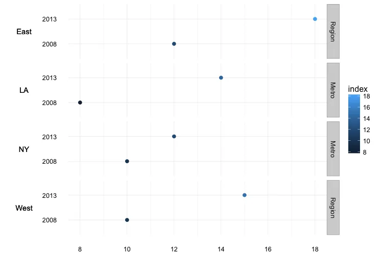
dt <- data.table(
value = c("East", "West","East", "West", "NY", "LA","NY", "LA"),
year = c(2008, 2008, 2013, 2013, 2008, 2008, 2013, 2013),
index = c(12, 10, 18, 15, 10, 8, 12 , 14),
var = c("Region","Region","Region","Region", "Metro","Metro","Metro","Metro"))
dt[, var := factor(var, levels=c( "Region", "Metro"))]
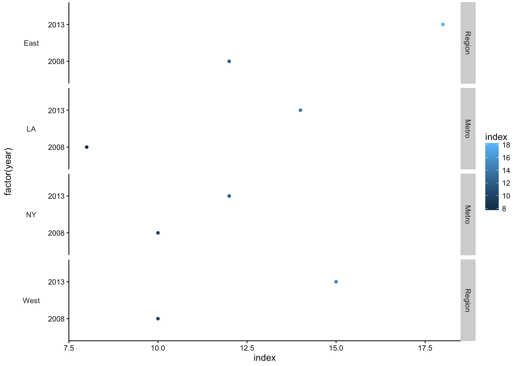
ggplot(data=dt) +
geom_point( aes(x=index, y= factor(year), color=index)) +
facet_grid(value + var ~., scales = "free_y", space="free") +
theme_bw() +
theme(panel.grid=element_blank()) +
theme(panel.border=element_blank()) +
theme(axis.line.x=element_line()) +
theme(axis.line.y=element_line()) -> gg
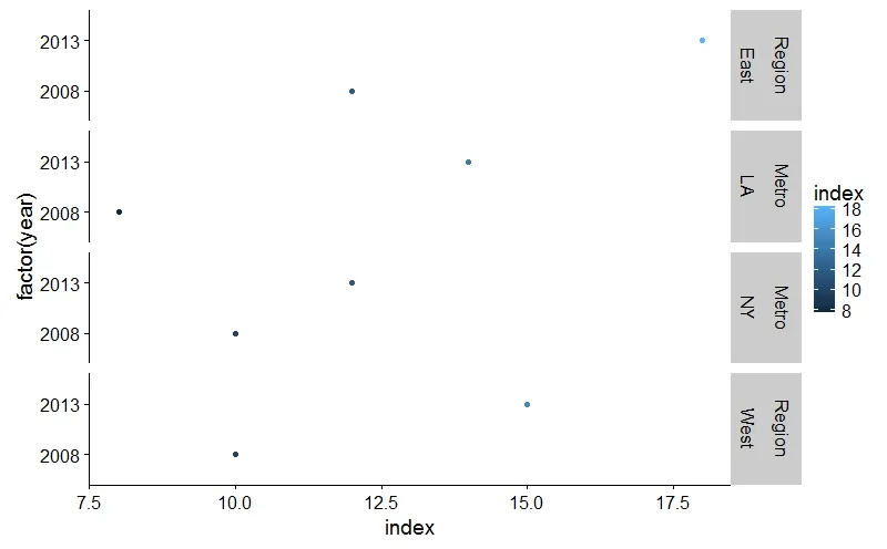
gb <- ggplot_build(gg)
gt <- ggplot_gtable(gb)
以下是其样式:
gt
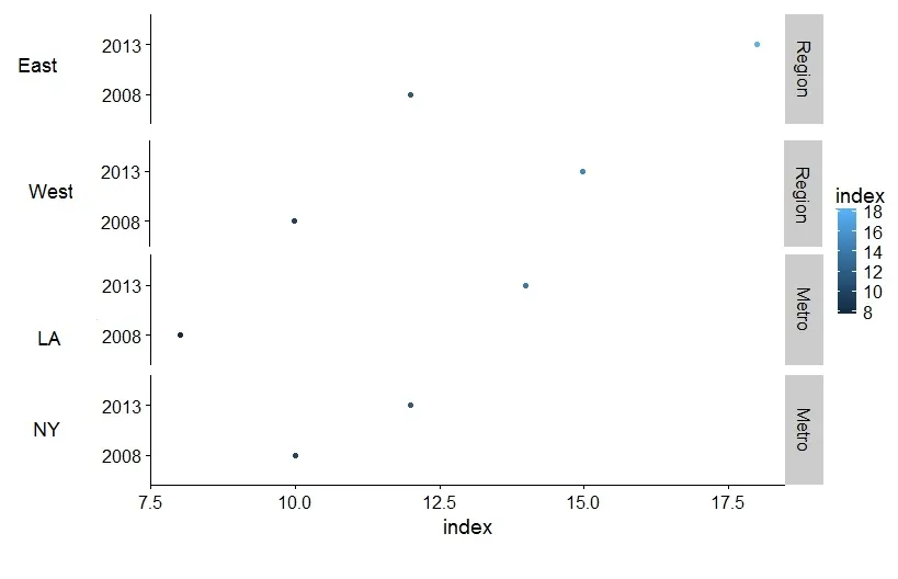
我们可以轻松地操作这些组件:
gt2 <- gt
gt2 <- gtable_add_cols(gt2, unit(3.0, "lines"), 2)
for_left <- gt[c(4,6,8,10),5]
gt2 <- gtable_add_grob(gt2, for_left$grobs[[1]], t=4, l=3, b=4, r=3)
gt2 <- gtable_add_grob(gt2, for_left$grobs[[2]], t=6, l=3, b=6, r=3)
gt2 <- gtable_add_grob(gt2, for_left$grobs[[3]], t=8, l=3, b=8, r=3)
gt2 <- gtable_add_grob(gt2, for_left$grobs[[4]], t=10, l=3, b=10, r=3)
gt2 <- gt2[, -6]
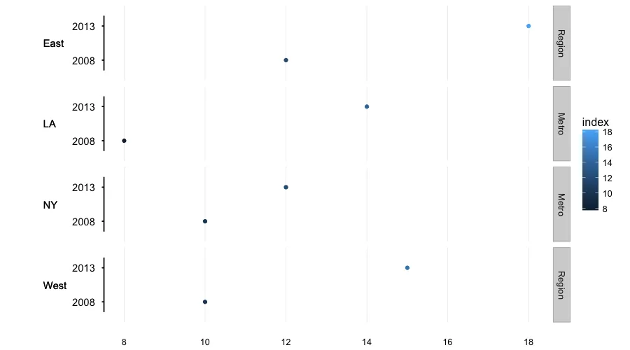
for (gi in 21:24) {
gt2$grobs[[gi]]$children[[1]]$gp$fill <- "white"
gt2$grobs[[gi]]$children[[1]]$gp$col <- "white"
gt2$grobs[[gi]]$children[[2]]$children[[1]]$rot <- 0
}
grid.arrange(gt2)
在我看来,第一个回答中的自定义标签和geom_text方法更易读并且更容易重复使用。
geom_text和geom_segment的答案。再次感谢! - rafa.pereira