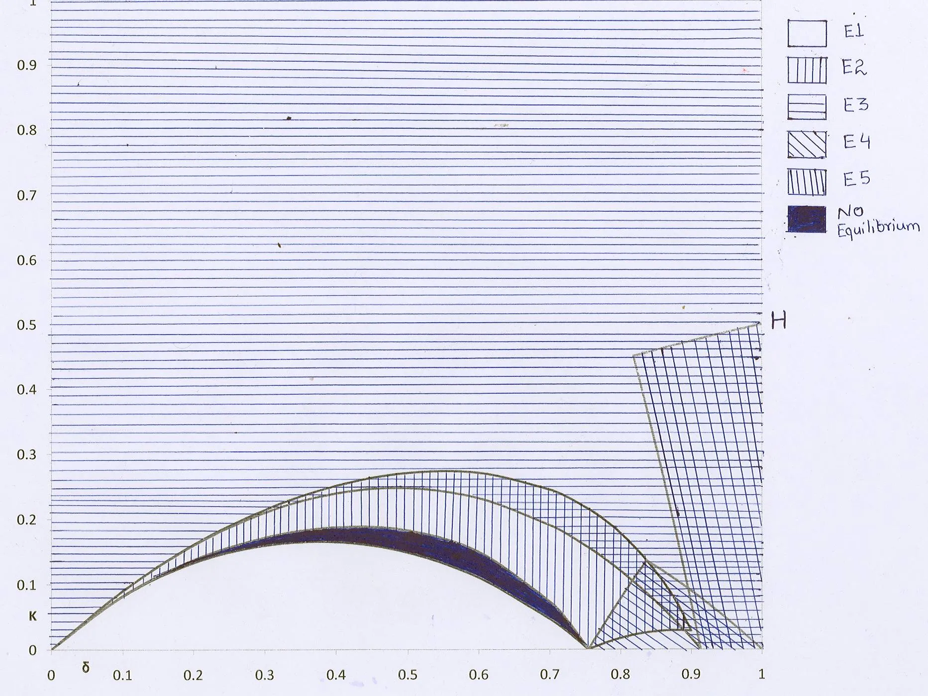
参考上面的图。我已经在Excel中绘制了方程,然后手动着色。你可以看到它不是很整洁。你可以看到有六个区域,每个区域由两个或多个方程界定。如何使用斜线图案画出不等式并阴影化区域,这是最简单的方法?
参考上面的图。我已经在Excel中绘制了方程,然后手动着色。你可以看到它不是很整洁。你可以看到有六个区域,每个区域由两个或多个方程界定。如何使用斜线图案画出不等式并阴影化区域,这是最简单的方法?
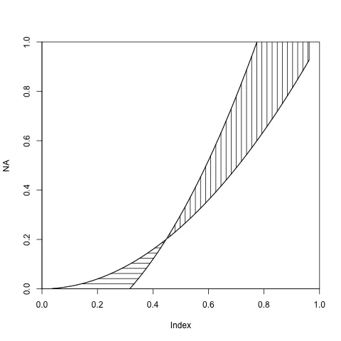
在 @agstudy 的回答基础上,以下是一种快速且简单的方法来表示R中的不等式:
plot(NA,xlim=c(0,1),ylim=c(0,1), xaxs="i",yaxs="i") # Empty plot
a <- curve(x^2, add = TRUE) # First curve
b <- curve(2*x^2-0.2, add = TRUE) # Second curve
names(a) <- c('xA','yA')
names(b) <- c('xB','yB')
with(as.list(c(b,a)),{
    id <- yB<=yA
    # b<a area
    polygon(x = c(xB[id], rev(xA[id])),
            y = c(yB[id], rev(yA[id])),
            density=10, angle=0, border=NULL)
    # a>b area
    polygon(x = c(xB[!id], rev(xA[!id])),
            y = c(yB[!id], rev(yA[!id])),
            density=10, angle=90, border=NULL)
    })
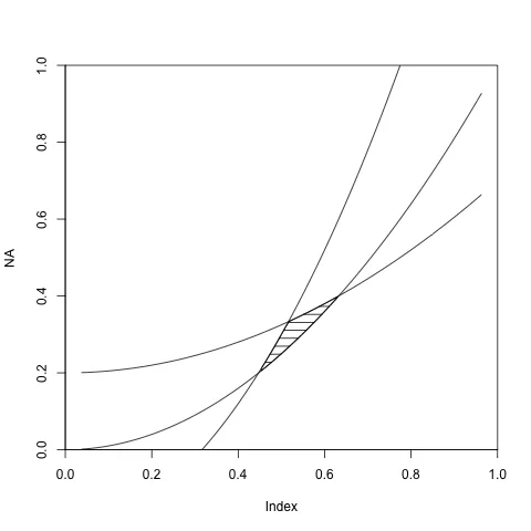
如果所涉及的区域被超过两个方程式所包围,则只需添加更多条件:
plot(NA,xlim=c(0,1),ylim=c(0,1), xaxs="i",yaxs="i") # Empty plot
a <- curve(x^2, add = TRUE) # First curve
b <- curve(2*x^2-0.2, add = TRUE) # Second curve
d <- curve(0.5*x^2+0.2, add = TRUE) # Third curve

names(a) <- c('xA','yA')
names(b) <- c('xB','yB')
names(d) <- c('xD','yD')

with(as.list(c(a,b,d)),{
    # Basically you have three conditions:
    # curve a is below curve b, curve b is below curve d and curve d is above curve a
    # assign to each curve coordinates the two conditions that concerns it.

    idA <- yA<=yD & yA<=yB
    idB <- yB>=yA & yB<=yD
    idD <- yD<=yB & yD>=yA
    polygon(x = c(xB[idB], xD[idD], rev(xA[idA])),
            y = c(yB[idB], yD[idD], rev(yA[idA])),
            density=10, angle=0, border=NULL)
    })
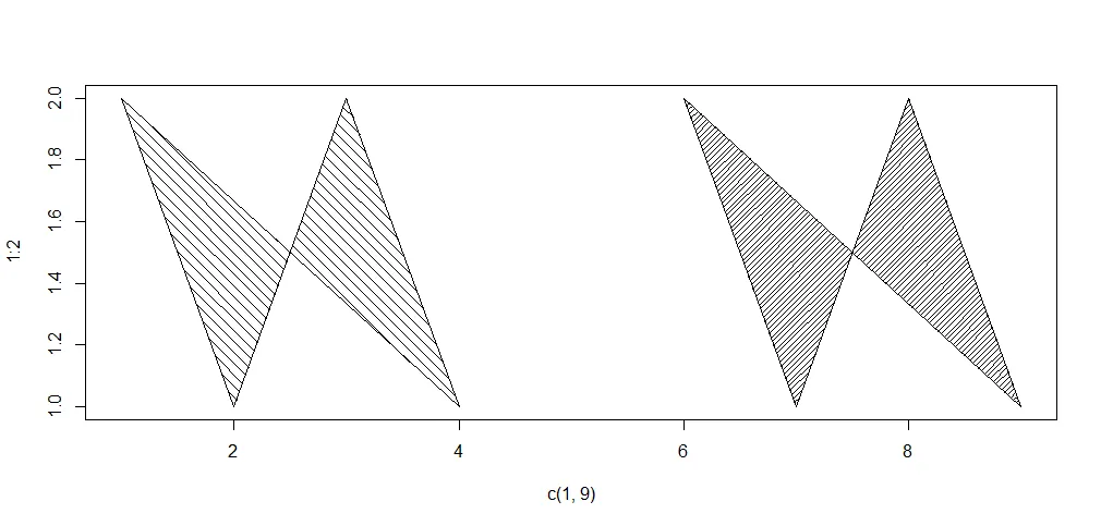
curve返回已绘制点的坐标是R版本2.10.0的新功能之一。 - plannapusggplot2或lattice。plot(c(1, 9), 1:2, type = "n")
polygon(1:9, c(2,1,2,1,NA,2,1,2,1),
density = c(10, 20), angle = c(-45, 45))
编辑
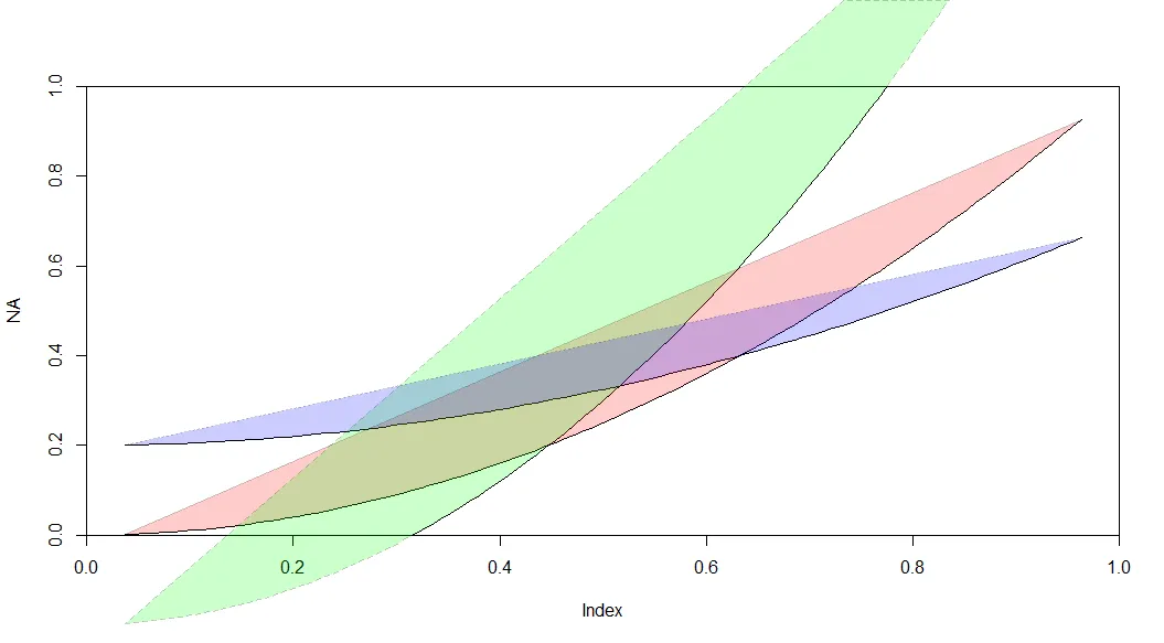
另一种选择是使用alpha混合来区分区域。在这里,使用@plannapus的示例和gridBase包来叠加多边形,您可以做出类似以下的效果:
library(gridBase)
vps <- baseViewports()
pushViewport(vps$figure,vps$plot)
with(as.list(c(a,b,d)),{
  grid.polygon(x = xA, y = yA,gp =gpar(fill='red',lty=1,alpha=0.2))
  grid.polygon(x = xB, y = yB,gp =gpar(fill='green',lty=2,alpha=0.2))
  grid.polygon(x = xD, y = yD,gp =gpar(fill='blue',lty=3,alpha=0.2))
}
)
upViewport(2)