Matlab：在两个曲线之间绘制面积，这两个曲线的值是依赖于曲线本身的。

Question

我正试图根据曲线的值来填充两条曲线之间的区域，这涉及到一个依赖于曲线值的函数。

这是我目前为止所做的代码：

    i=50;
cc = @(xx,x,y) 1./(1+(exp(-xx)/(exp(-x)-exp(-y))));
n_vec = 2:0.1:10;
x_vec = linspace(2,10,length(n_vec));
y_vec = abs(sin(n_vec));
N=[n_vec,fliplr(n_vec)];  
X=[x_vec,fliplr(y_vec)];
figure(1)
subplot(2,1,1)
hold on
plot(n_vec,x_vec,n_vec,y_vec)
hp = patch(N,X,'b')
plot([n_vec(i) n_vec(i)],[x_vec(i),y_vec(i)],'linewidth',5)
xlabel('n'); ylabel('x')
subplot(2,1,2)

xx = linspace(y_vec(i),x_vec(i),100);
plot(xx,cc(xx,y_vec(i),x_vec(i)))
xlabel('x'); ylabel('c(x)')

这段代码生成以下的图形：

我添加了颜色编码，用于表示每条线（沿着x轴上的一个点在y轴上）在两条曲线之间的区域所应有的颜色编码。

总体来说，整个区域应该被填充上取决于曲线值的渐变颜色。

我协助了以下之前的问题，但无法解决：

MATLAB 填充两条线之间的区域

使用渐变颜色填充圆形

根据 MATLAB 函数给定的颜色映射填充两条曲线之间的区域

注意：曲线的函数形式不重要，我更喜欢参考由两个一般数组组成的曲线的答案。

- jarhead

Answer 1

浏览器绘图方法

1. 与散点图方法相同，即生成一个点网格。

y = [x_vec(:); y_vec(:)];
resolution = [500,500];
px = linspace(min(n_vec), max(n_vec), resolution(1));
py = linspace(min(y), max(y), resolution(2));
[px, py] = meshgrid(px, py);

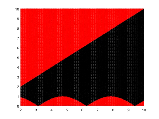
生成一个逻辑数组，指示点是否在多边形内部，但不需要提取这些点：

in = inpolygon(px, py, N, X);

生成Z。Z的值表示曲面图使用的颜色。因此，应使用您的函数cc生成它。

pz = 1./(1+(exp(-py_)/(exp(-y_vec(i))-exp(-x_vec(i)))));
pz = repmat(pz',1,resolution(2));

4. 将区域外的点的 Z 值设置为 NaN，以便 MATLAB 不会绘制它们。

pz(~in) = nan;

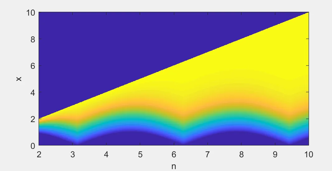
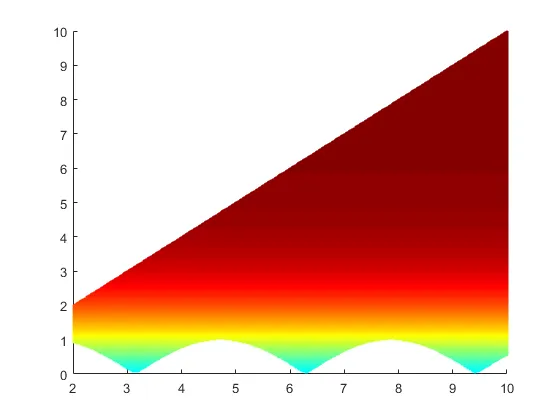
生成一个有界的颜色映射（如果要使用完整的颜色范围，请删除）

% generate colormap
c = jet(100);
[s,l] = bounds(pz,'all');
s = round(s*100);
l = round(l*100);
if s ~= 0
    c(1:s,:) = [];
end
if l ~= 100
    c(l:100,:) = [];
end

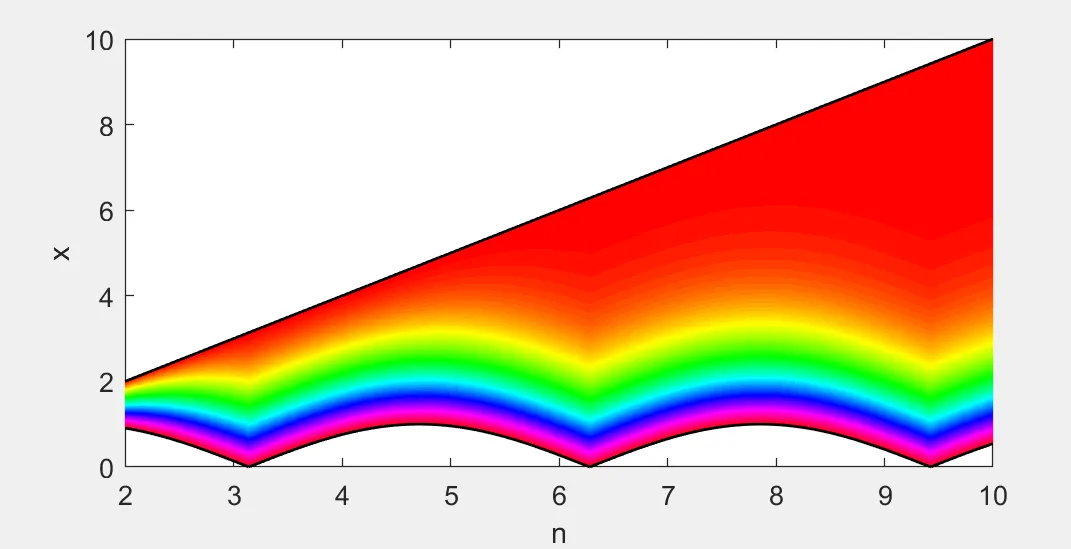
最后，绘制图表。

figure;
colormap(jet)
surf(px,py,pz,'edgecolor','none');
view(2) % x-y view

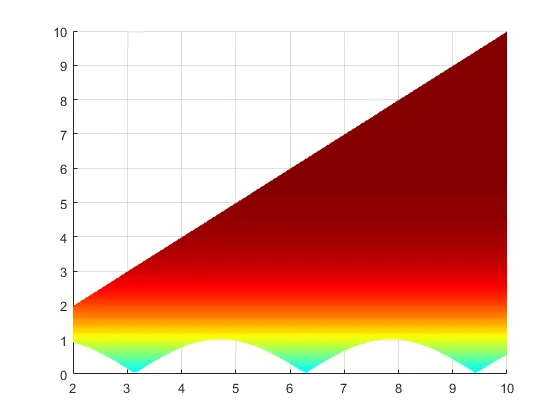
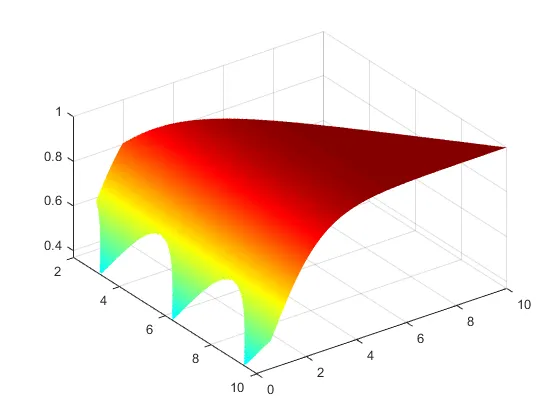
随意旋转图像，看看在Z维度中的样子 - 美丽 :)

---

测试的完整代码：

i=50;
cc = @(xx,x,y) 1./(1+(exp(-xx)/(exp(-x)-exp(-y))));
n_vec = 2:0.1:10;
x_vec = linspace(2,10,length(n_vec));
y_vec = abs(sin(n_vec));

% generate grid
y = [x_vec(:); y_vec(:)];
resolution = [500,500];
px_ = linspace(min(n_vec), max(n_vec), resolution(1));
py_ = linspace(min(y), max(y), resolution(2));
[px, py] = meshgrid(px_, py_);

% extract points
in = inpolygon(px, py, N, X);

% generate z
pz = 1./(1+(exp(-py_)/(exp(-y_vec(i))-exp(-x_vec(i)))));
pz = repmat(pz',1,resolution(2));
pz(~in) = nan;

% generate colormap
c = jet(100);
[s,l] = bounds(pz,'all');
s = round(s*100);
l = round(l*100);
if s ~= 0
    c(1:s,:) = [];
end
if l ~= 100
    c(l:100,:) = [];
end

% plot
figure;
colormap(c)
surf(px,py,pz,'edgecolor','none');
view(2)

- Anthony

Answer 2

你可以使用imagesc和meshgrids。请查看代码中的注释以了解发生了什么。

将数据进行降采样。

% your initial upper and lower boundaries
n_vec_long = linspace(2,10,1000000);

f_ub_vec_long = linspace(2, 10, length(n_vec_long));
f_lb_vec_long = abs(sin(n_vec_long));

% downsample
n_vec = linspace(n_vec_long(1), n_vec_long(end), 1000); % for example, only 1000 points

% get upper and lower boundary values for n_vec
f_ub_vec = interp1(n_vec_long, f_ub_vec_long, n_vec); 
f_lb_vec = interp1(n_vec_long, f_lb_vec_long, n_vec); 

% x_vec for the color function
x_vec = 0:0.01:10;

绘制数据。

% create a 2D matrix with N and X position
[N, X] = meshgrid(n_vec, x_vec);

% evaluate the upper and lower boundary functions at n_vec
% can be any function at n you want (not tested for crossing boundaries though...)
f_ub_vec = linspace(2, 10, length(n_vec));
f_lb_vec = abs(sin(n_vec));

% make these row vectors into matrices, to create a boolean mask
F_UB = repmat(f_ub_vec, [size(N, 1) 1]);
F_LB = repmat(f_lb_vec, [size(N, 1) 1]);

% create a mask based on the upper and lower boundary functions
mask = true(size(N));
mask(X > F_UB | X < F_LB) = false;

% create data matrix
Z = NaN(size(N));

% create function that evaluates the color profile for each defined value 
% in the vectors with the lower and upper bounds
zc = @(X, ub, lb) 1 ./ (1 + (exp(-X) ./ (exp(-ub) - exp(-lb))));
CData = zc(X, f_lb_vec, f_ub_vec); % create the c(x) at all X

% put the CData in Z, but only between the lower and upper bound.
Z(mask) = CData(mask);

% normalize Z along 1st dim
Z = normalize(Z, 1, 'range'); % get all values between 0 and 1 for colorbar

% draw a figure!
figure(1); clf;
ax = axes;                          % create some axes
sc = imagesc(ax, n_vec, x_vec, Z);  % plot the data
ax.YDir = 'normal' % set the YDir to normal again, imagesc reverses it by default;

xlabel('n')
ylabel('x')

这已经有点像你想要的了，但是让我们消除边界外的蓝色区域。这可以通过创建一个“alpha遮罩”来实现，即将所有位于先前定义的mask之外的像素的alpha值设置为0：

figure(2); clf;
ax = axes;                          % create some axes
hold on;
sc = imagesc(ax, n_vec, x_vec, Z);  % plot the data
ax.YDir = 'normal' % set the YDir to normal again, imagesc reverses it by default;

% set a colormap 
colormap(flip(hsv(100)))

% set alpha for points outside mask
Calpha = ones(size(N));
Calpha(~mask) = 0;
sc.AlphaData = Calpha;

% plot the other lines
plot(n_vec, f_ub_vec, 'k', n_vec, f_lb_vec, 'k' ,'linewidth', 1)

% set axis limits
xlim([min(n_vec), max(n_vec)])
ylim([min(x_vec), max(x_vec)])

- rinkert

---

谢谢您的回答，但这并没有对我有太大帮助。首先，该代码无法应用于大型数据集。其次，也是最重要的一点，颜色渐变应仅在两条曲线之间的区域内。这意味着两条曲线之间的距离定义了渐变的锐度。在您的结果中，所有n值的情况都是相同的。 - jarhead

@jarhead 我明白了，目前只使用了下边界。你能否在问题中展示你想要使用的数据集的类型（维度、生成样本数据的代码等）？ - rinkert

编写代码并不会有什么不同，考虑将其应用于长度约为1000000的向量。网格对内存来说太大了，也许使用patch命令会更好？ - jarhead

@jarhead，确实将此应用于那么长的向量是行不通的，但你在屏幕上也没有那么多像素，因此无论如何都看不到细节。您可以对数据进行插值/下采样，我会将其添加到答案中。 - rinkert

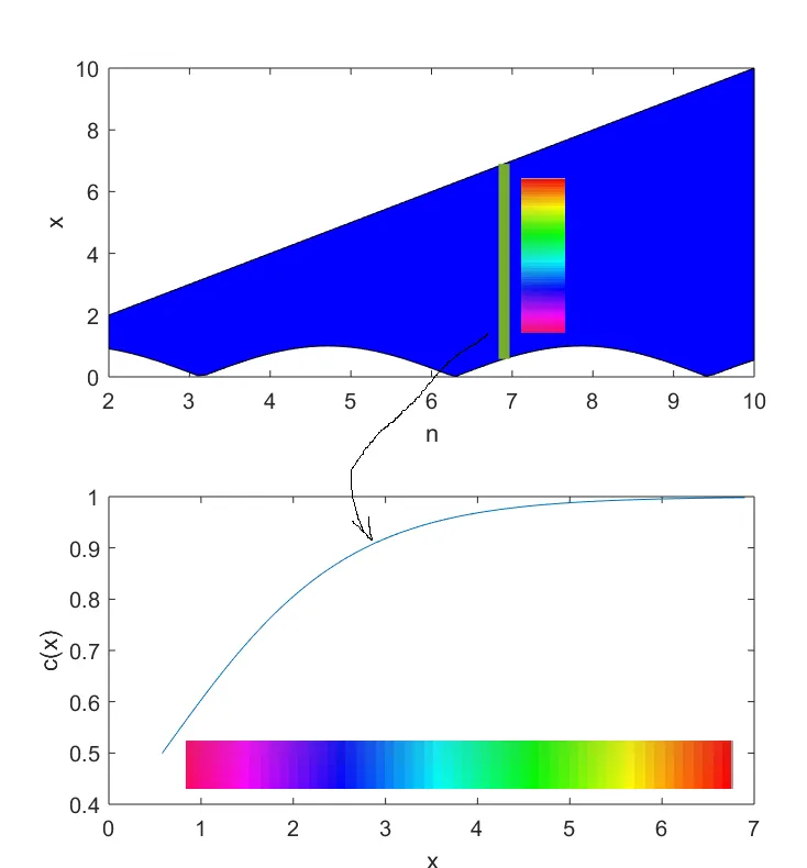
我认为patch只允许在边缘的颜色值之间进行线性插值，因此无法满足您对c(x)颜色函数的要求。 - rinkert

Answer 3

曲线的函数形式并不重要，我更喜欢一个回答，它涉及到由曲线组成的两个通用数组。

使用patch实现这一点很困难。

但是，您可以使用散点图来用彩色点“填充”区域。或者，更好的方法是使用surf绘图，并使用您的cc函数生成z坐标（请参见我的单独解决方案）。

散点图方法

1. 首先，在包围两条曲线的矩形空间内创建一个点网格（分辨率为500*500）。

y = [x_vec(:); y_vec(:)];
resolution = [500,500];
px = linspace(min(n_vec), max(n_vec), resolution(1));
py = linspace(min(y), max(y), resolution(2));
[px, py] = meshgrid(px, py);

figure; 
scatter(px(:), py(:), 1, 'r');

点网格的不太有趣的图形：

2. 接下来，提取由两条曲线定义的多边形内部的点。

in = inpolygon(px, py, N, X);
px = px(in);
py = py(in);

hold on;
scatter(px, py, 1, 'k');

黑点在区域内：

3. 最后，创建颜色并绘制漂亮的渐变色图。

% create color for the points
cid = 1./(1+(exp(-py)/(exp(-y_vec(i))-exp(-x_vec(i)))));
c = jet(101);
c = c(round(cid*100)+1,:); % +1 to avoid zero indexing

% plot
figure;
scatter(px,py,16,c,'filled','s'); % use size 16, filled square markers.

请注意，您可能需要一个相当密集的点网格来确保白色背景不会显示出来。您也可以将点大小更改为较大的值（不会影响性能）。

当然，您可以使用patch替换scatter，但您需要计算出顶点和面ID，然后您可以使用patch('Faces',F,'Vertices',V)单独修补每个面。以这种方式使用patch可能会影响性能。

---

用于测试的完整代码：

i=50;
cc = @(xx,x,y) 1./(1+(exp(-xx)/(exp(-x)-exp(-y))));
n_vec = 2:0.1:10;
x_vec = linspace(2,10,length(n_vec));
y_vec = abs(sin(n_vec));

% generate point grid
y = [x_vec(:); y_vec(:)];
resolution = [500,500];
px_ = linspace(min(n_vec), max(n_vec), resolution(1));
py_ = linspace(min(y), max(y), resolution(2));
[px, py] = meshgrid(px_, py_);

% extract points
in = inpolygon(px, py, N, X);
px = px(in);
py = py(in);


% generate color
cid = 1./(1+(exp(-py)/(exp(-y_vec(i))-exp(-x_vec(i)))));
c = jet(101);
c = c(round(cid*100)+1,:); % +1 to avoid zero indexing

% plot
figure;
scatter(px,py,16,c,'filled','s');

- Anthony