这不是一个琐碎的问题。它需要编写一个新的
Geom,一个新的
Stat和一个新的
Grob(见下文)。我个人并不认为这是一个很好的数据可视化选项,因为它会扭曲位置并引起显著的舍入误差。然而,它在视觉上很吸引人且相当直观,所以我还是写了一个
geom_hextri。要使其正常工作,我们只需将其美学映射到一个分类变量上,它应该能够按预期运行。
让我们使用您自己的示例数据:
set.seed(1)
n = 100

df = data.frame(x = rnorm(n),
                y = rnorm(n),
                group = sample(0:1, n, prob = c(0.9, 0.1), replace = TRUE))
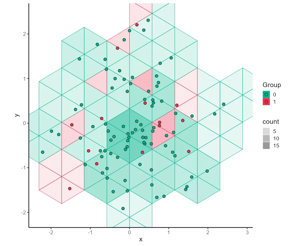
使用您选择的颜色方案,用
geom_hextri绘制它。我们将叠加点以确保段填充的逻辑与点匹配。
ggplot(df, aes(x, y, fill = factor(group), color = factor(group))) +
  geom_hextri(linewidth = 0.3, bins = 4) +
  geom_point(shape = 21, size = 3, color = "black") +
  coord_equal() +
  theme_classic(base_size = 16) +
  theme(aspect.ratio = 1) +
  scale_fill_manual("Group", values =  c("#00b38a", "#ea324c")) +
  scale_color_manual("Group", values =  c("#00b38a", "#ea324c"))
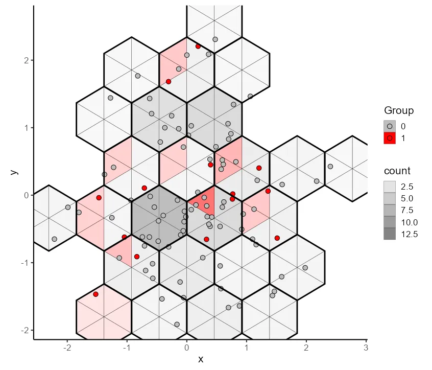
请注意,如果我们需要的话,更改箱子大小和美学非常容易。为了在我们的三角形周围得到实心的六边形,我们只需添加一个
geom_hex图层:
ggplot(df, aes(x, y, fill = factor(group))) +
  geom_hextri(color = "black", linewidth = 0.1, bins = 5) +
  geom_point(shape = 21, size = 3) +
  geom_hex(fill = NA, color = "black", linewidth = 1, bins = 5) +
  coord_equal() +
  theme_classic(base_size = 16) +
  theme(aspect.ratio = 1) +
  scale_fill_manual("Group", values = c("gray", "red"))
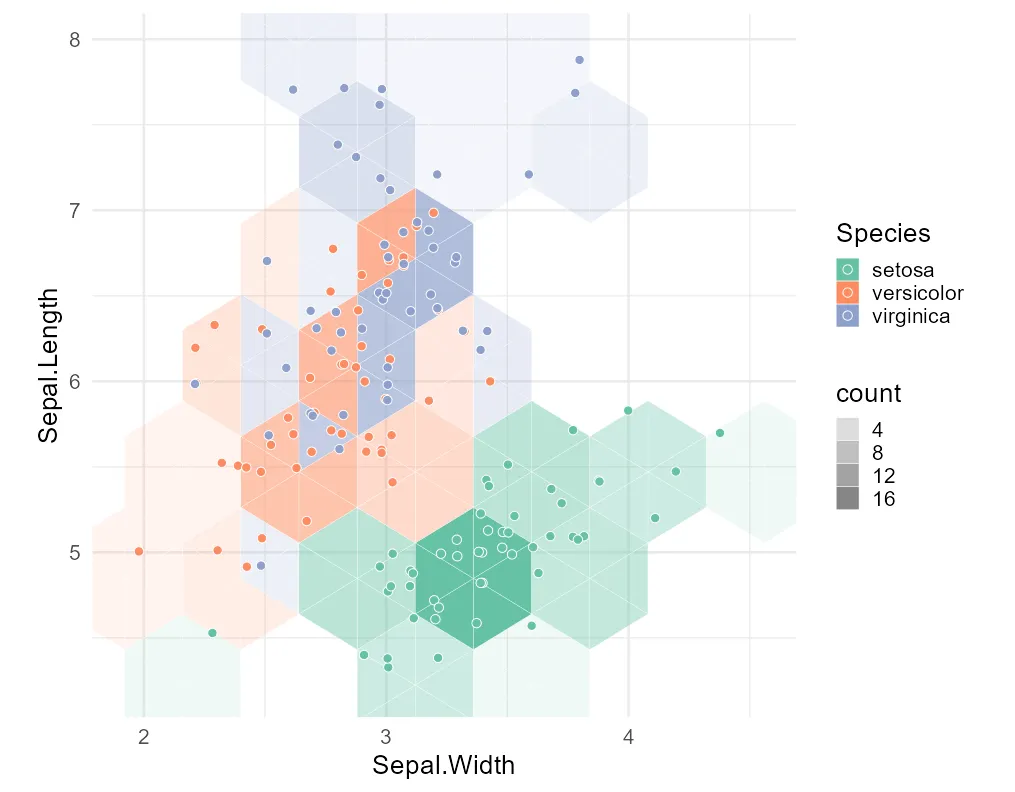
应用于另一个数据集,我们得到:
ggplot(iris, aes(Sepal.Width, Sepal.Length, fill = Species)) +
  geom_hextri(color = "white", linewidth = 0.1, bins = 5) +
  geom_point(shape = 21, size = 3, position = position_jitter(0.03, 0.03),
             color = "white") +
  geom_hex(fill = NA, colour = NA, linewidth = 1, bins = 5) +
  coord_equal() +
  theme_minimal(base_size = 20) +
  theme(aspect.ratio = 1) +
  scale_fill_brewer(palette = "Set2")
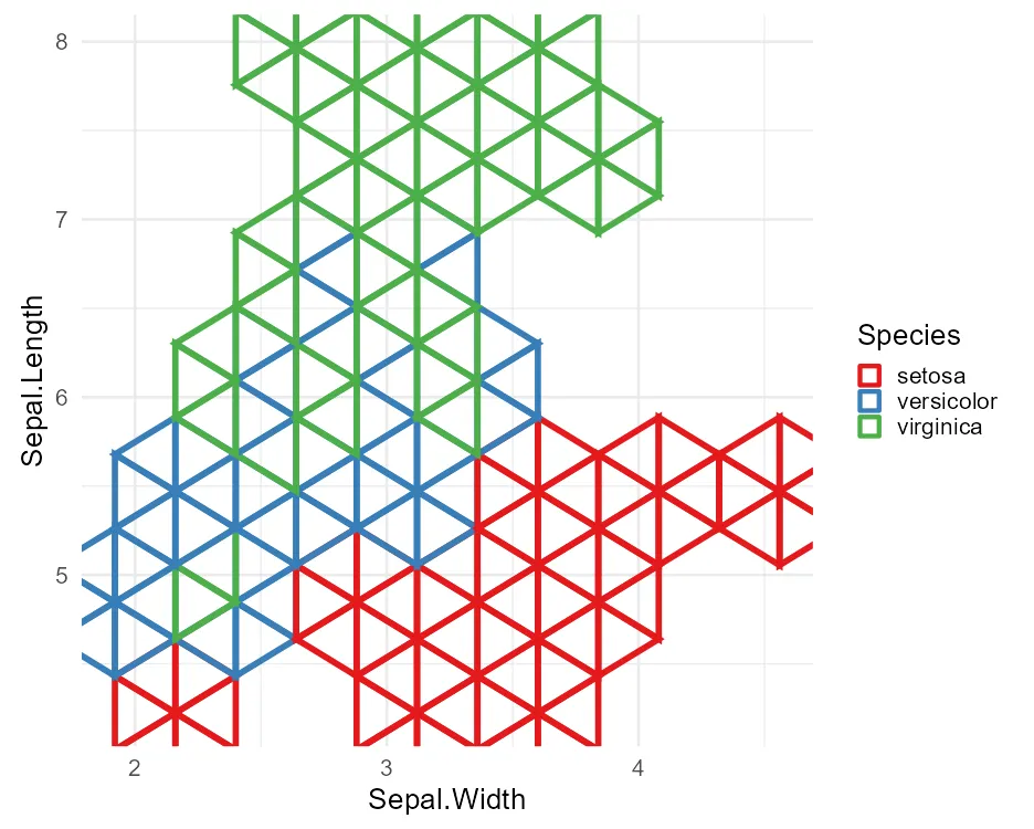
请注意,我们不需要使用填充美学。例如,我们可以简单地更改轮廓颜色。
ggplot(iris, aes(Sepal.Width, Sepal.Length, colour = Species)) +
  geom_hextri(fill = NA, linewidth = 2, bins = 5, alpha = 1) +
  geom_hex(fill = NA, colour = NA, linewidth = 1, bins = 5) +
  coord_equal() +
  theme_minimal(base_size = 20) +
  theme(aspect.ratio = 1) +
  scale_colour_brewer(palette = "Set1")
geom_hextri代码
现在是困难的部分 - 实现
geom_hextri。我尝试将其分解成块,但代码必然很长,而且很难以详细解释。为了适应不需要滚动的代码框,我也不得不稍微牺牲一些间距。
最终,ggplot必须将对象作为图形对象(grobs)绘制在绘图设备上,但是目前没有现成的grob可以绘制这些六边形片段,因此我们需要定义一个函数来使用grid::polygonGrob绘制它们,给定适当的x、y坐标、高度、宽度、图形参数和我们正在处理的片段。这个函数需要接受向量化的数据以便与ggplot一起使用。
hextriGrob <- function(x, y, seg, height, width, gp = grid::gpar()) {

  gp <- lapply(seq_along(x), function(i) structure(gp[i], class = "gpar"))
  xl  <- x - width
  xr  <- x + width
  y1  <- y + 2 * height
  y2  <- y + height
  y3  <- y - height
  y4  <- y - 2 * height
  pg  <- grid::polygonGrob

  do.call(grid::gList,
    Map(function(x, y, xl, xr, y1, y2, y3, y4, seg, gp) {
      if(seg == 1) return(pg(x = c(x, x, xr, x),  y = c(y, y1, y2, y), gp = gp))
      if(seg == 2) return(pg(x = c(x, xr, xr, x), y = c(y, y2, y3, y), gp = gp))
      if(seg == 3) return(pg(x = c(x, xr, x, x),  y = c(y, y3, y4, y), gp = gp))
      if(seg == 4) return(pg(x = c(x, x, xl, x),  y = c(y, y4, y3, y), gp = gp))
      if(seg == 5) return(pg(x = c(x, xl, xl, x), y = c(y, y3, y2, y), gp = gp))
      if(seg == 6) return(pg(x = c(x, xl, x, x),  y = c(y, y2, y1, y), gp = gp))
  }, x = x, y = y, xl = xl, xr = xr, y1 = y1,
     y2 = y2, y3 = y3, y4 = y4, seg = seg, gp = gp))
}
但这本身还不够。我们还需要定义一个继承自GeomHex的geom,但它有自己的compute_group方法来适当地调用我们的hextriGrob函数。它的一部分工作将是确保美学正确地拆分为片段,由于技术原因,并不是所有的拆分都可以在Stat层中轻松完成。
GeomHextri <- ggproto("GeomHextri", GeomHex,
  draw_group = function (self, data, panel_params, coord, lineend = "butt",
                         linejoin = "mitre", linemitre = 10) {
    table_six <- function(vec) {
      if(!is.factor(vec)) vec <- factor(vec)
      tab <- round(6 * table(vec, useNA = "always")/length(vec))
      n <- diff(c(0, findInterval(cumsum(tab) / sum(tab), 1:6/6)))
      rep(names(tab), times = n)
    }
    num_cols <- sapply(data, is.numeric)
    non_num_cols <- names(data)[!num_cols]
    num_cols <- names(data)[num_cols]
    datasplit <- split(data, interaction(data$x, data$y, drop = TRUE))
    data <- do.call("rbind", lapply(seq_along(datasplit), function(i) {
      num_list <- lapply(datasplit[[i]][num_cols], function(x) rep(mean(x), 6))
      non_num_list <- lapply(datasplit[[i]][non_num_cols], function(x) {
        table_six(rep(x, times = datasplit[[i]]$count))})
      d <- datasplit[[i]][rep(1, 6),]
      d[num_cols] <- num_list
      d[non_num_cols] <- non_num_list
      d$tri <- 1:6
      d$group <- i
      d}))
    data <- ggplot2:::check_linewidth(data, snake_class(self))
    if (ggplot2:::empty(data))  return(zeroGrob())
    coords <- coord$transform(data, panel_params)
    hw <- c(min(diff(unique(sort(coords$x)))),
            min(diff(unique(sort(coords$y))))/3)
    hextriGrob(coords$x, coords$y, data$tri, hw[2], hw[1],
      gp = grid::gpar(col = data$colour, fill = alpha(data$fill, data$alpha),
                      lwd = data$linewidth * .pt, lty = data$linetype,
                      lineend = lineend, linejoin = linejoin,
                      linemitre = linemitre))})
在我们的数据传送到这个几何图形之前,它需要被分成六边形的区块。不幸的是,现有的StatBinhex无法在保留我们所需的每个段落级别美学细节的同时完成此操作,因此我们必须编写自己的分块函数:
hexify <- function (x, y, z, xbnds, ybnds, xbins, ybins, binwidth,
                    fun = mean, fun.args = list(),
                    drop = TRUE) {

  hb <- hexbin::hexbin(x, xbnds = xbnds, xbins = xbins, y,
                       ybnds = ybnds, shape = ybins/xbins, IDs = TRUE)
  value <- rlang::inject(tapply(z, hb@cID, fun, !!!fun.args))
  out <- hexbin::hcell2xy(hb)
  out <- ggplot2:::data_frame0(!!!out)
  out$value <- as.vector(value)
  out$width <- binwidth[1]
  out$height <- binwidth[2]
  if (drop) out <- stats::na.omit(out)
  out
}
这个然后必须在自定义的Stat内部使用:
StatHextri <- ggproto("StatBinhex", StatBinhex,
  default_aes = aes(weight = 1, alpha = after_stat(count)),
  compute_panel = function (self, data, scales, ...) {
    if (ggplot2:::empty(data)) return(ggplot2:::data_frame0())
    data$group <- 1
    self$compute_group(data = data, scales = scales, ...)},
  compute_group = function (data, scales, binwidth = NULL, bins = 30,
                            na.rm = FALSE){
    `%||%` <- rlang::`%||%`
    rlang::check_installed("hexbin", reason = "for `stat_binhex()`")
    binwidth <- binwidth %||% ggplot2:::hex_binwidth(bins, scales)
    if (length(binwidth) == 1) binwidth <- rep(binwidth, 2)
    wt <- data$weight %||% rep(1L, nrow(data))
    non_pos <- !names(data) %in% c("x", "y", "PANEL", "group")
    is_num  <- sapply(data, is.numeric)
    aes_vars <- names(data)[non_pos & !is_num]
    grps <- do.call("interaction", c(as.list(data[aes_vars]), drop = TRUE))
    xbnds <- ggplot2:::hex_bounds(data$x, binwidth[1])
    xbins <- diff(xbnds)/binwidth[1]
    ybnds <- ggplot2:::hex_bounds(data$y, binwidth[2])
    ybins <- diff(ybnds)/binwidth[2]
    do.call("rbind", Map(function(data, wt) {
      out <- hexify(data$x, data$y, wt, xbnds, ybnds, xbins,
                    ybins, binwidth, sum)
      for(var in aes_vars) out[[var]] <- data[[var]][1]
      out$density <- as.vector(out$value/sum(out$value, na.rm = TRUE))
      out$ndensity <- out$density/max(out$density, na.rm = TRUE)
      out$count <- out$value
      out$ncount <- out$count/max(out$count, na.rm = TRUE)
      out$value <- NULL
      out$group <- 1
      out}, split(data, grps), split(wt, grps)))})
最后,我们需要编写一个几何函数,这样我们才能在 ggplot 调用中轻松调用上述所有内容。
geom_hextri <- function(
    mapping     = aes(),
    data        = NULL,
    stat        = "hextri",
    position    = "identity",
    na.rm       = FALSE,
    show.legend = NA,
    inherit.aes = TRUE,
    bins        = 10,
    ...) {

      ggplot2::layer(
        geom        = GeomHextri,
        data        = data,
        mapping     = mapping,
        stat        = stat,
        position    = position,
        show.legend = show.legend,
        inherit.aes = inherit.aes,
        params      = list(na.rm = na.rm, bins = bins, ...)
      )
  }
Geom和可能还有一个Stat,以及调用它们的函数。可能还需要编写一个基于多边形grob的新的grob类型,以可靠地绘制三角形。当所有这些都被编写完成时,最好将其放入一个R包中。这是一项庞大的工作,特别是对于一个有些小众(而且,我敢说,不直观)的数据可视化任务来说。对于一个Stack Overflow回答来说,这可能是太多的工作了,即使有赏金也是如此。但我希望我是错的... - Allan CameronGeom和可能还有一个Stat,以及调用它们的函数。可能还需要编写一个基于多边形grob的新grob类型,以可靠地绘制三角形。当所有这些都被编写完成时,最好将其放入一个R包中。这是一项庞大的工作,尤其对于一个有点小众(而且,我敢说,不直观)的数据可视化任务来说。即使有了悬赏,这也可能是太多的工作量,超出了Stack Overflow回答的范围。不过,我希望我是错的... - Allan Cameron