我曾经为MRI数据增强做过类似的事情:
可能代码可以被优化,但它现在就能工作。
我的数据是3维numpy数组,代表一个MRI扫描仪。它的大小为[128,128,128],但代码可以修改以接受任何维数。此外,当平面在立方体边界之外时,您必须在主函数中将变量fill赋默认值,在我的情况下我选择了:data_cube [0:5,0:5,0:5].mean()
def create_normal_vector(x, y,z):
normal = np.asarray([x,y,z])
normal = normal/np.sqrt(sum(normal**2))
return normal
def get_plane_equation_parameters(normal,point):
a,b,c = normal
d = np.dot(normal,point)
return a,b,c,d
def get_point_plane_proximity(plane,point):
return np.dot(plane[0:-1],point) - plane[-1]
def get_corner_interesections(plane, cube_dim = 128):
corners_list = []
only_x = np.zeros(4)
min_prox_x = 9999
min_prox_y = 9999
min_prox_z = 9999
min_prox_yz = 9999
for i in range(cube_dim):
temp_min_prox_x=abs(get_point_plane_proximity(plane,np.asarray([i,0,0])))
if temp_min_prox_x < min_prox_x:
min_prox_x = temp_min_prox_x
corner_intersection_x = np.asarray([i,0,0])
only_x[0]= i
temp_min_prox_y=abs(get_point_plane_proximity(plane,np.asarray([i,cube_dim,0])))
if temp_min_prox_y < min_prox_y:
min_prox_y = temp_min_prox_y
corner_intersection_y = np.asarray([i,cube_dim,0])
only_x[1]= i
temp_min_prox_z=abs(get_point_plane_proximity(plane,np.asarray([i,0,cube_dim])))
if temp_min_prox_z < min_prox_z:
min_prox_z = temp_min_prox_z
corner_intersection_z = np.asarray([i,0,cube_dim])
only_x[2]= i
temp_min_prox_yz=abs(get_point_plane_proximity(plane,np.asarray([i,cube_dim,cube_dim])))
if temp_min_prox_yz < min_prox_yz:
min_prox_yz = temp_min_prox_yz
corner_intersection_yz = np.asarray([i,cube_dim,cube_dim])
only_x[3]= i
corners_list.append(corner_intersection_x)
corners_list.append(corner_intersection_y)
corners_list.append(corner_intersection_z)
corners_list.append(corner_intersection_yz)
corners_list.append(only_x.min())
corners_list.append(only_x.max())
return corners_list
def get_points_intersection(plane,min_x,max_x,data_cube,shape=128):
fill = data_cube[0:5,0:5,0:5].mean()
extended_data_cube = np.ones([shape+2,shape,shape])*fill
extended_data_cube[1:shape+1,:,:] = data_cube
diag_image = np.zeros([shape,shape])
min_x_value = 999999
for i in range(shape):
for j in range(shape):
for k in range(int(min_x),int(max_x)+1):
current_value = abs(get_point_plane_proximity(plane,np.asarray([k,i,j])))
if current_value < min_x_value:
diag_image[i,j] = extended_data_cube[k,i,j]
min_x_value = current_value
min_x_value = 999999
return diag_image
它的工作方式如下:
你创建一个普通向量:
例如 [5,0,3]
normal1=create_normal_vector(5, 0,3)
然后你创建一个点:
(我的立方体数据形状为[128,128,128])
point = [64,64,64]
您可以计算平面方程的参数[a,b,c,d],其中ax+by+cz=d。
plane1=get_plane_equation_parameters(normal1,point)
然后为了减少搜索空间,您可以计算平面与立方体的交点:
corners1 = get_corner_interesections(plane1,128)
其中 corners1 = [intersection [x,0,0],intersection [x,128,0],intersection [x,0,128],intersection [x,128,128], min intersection [x,y,z], max intersection [x,y,z]]
有了这些,您可以计算立方体和平面之间的交点:
image1 = get_points_intersection(plane1,corners1[-2],corners1[-1],data_cube)
一些例子:
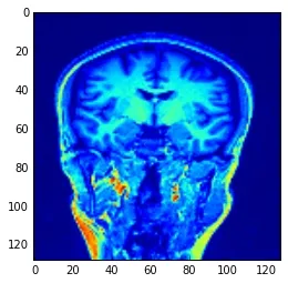
正常是[1,0,0],点是[64,64,64]。
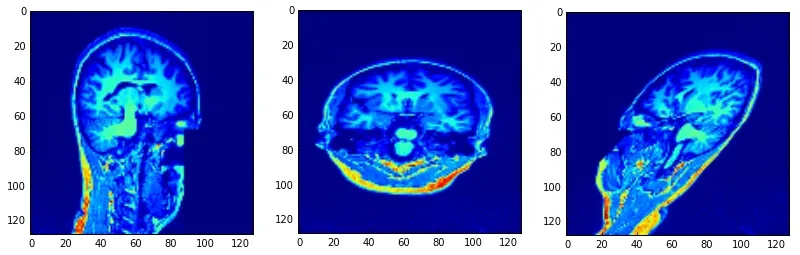
正常情况下是 [5,1,0],[5,1,1],[5,0,1],点为 [64,64,64]:

正常是 [5,3,0],[5,3,3],[5,0,3],点是 [64,64,64]:

正常是 [5,-5,0],[5,-5,-5],[5,0,-5] 点是 [64,64,64]:
谢谢。

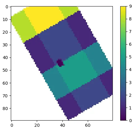
nan的有趣点。然而,这并不会告诉 matplotlib 关于补丁边界的信息。对我来说这很重要,因为如果你想发布类似的内容,最好有一个带有正确边界的图表。 - BandGap