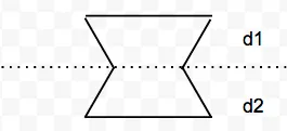
具有两个口的凹六边形的标准网格?
9
- Léo Léopold Hertz 준영
5个回答
3
例如,您可以查看Alexandra Baumgart和Hazuki Okuda使用Mathematica完成的示例。这是使用Manipulate实现的,有效地创建了基本的用户界面。
< p > < img alt="enter image description here" src="https://istack.dev59.com/pPOKQ.webp"/> < /p >
代码:
Manipulate[
Grid[{{Show[
ParametricPlot3D[{1.25Cos[t], 1.25 Sin[t],s+2-2w},{s,0,.25},{t,0,2Pi},PlotStyle->Directive[Opacity[1],Gray],Mesh->None, Lighting->"Neutral"],
ParametricPlot3D[{r Cos[t], r Sin[t],2.25-2w},{r,0,1.25},{t,0,2Pi},PlotStyle->Directive[Opacity[1],Gray],Mesh->None, Lighting->"Neutral"],
ParametricPlot3D[{r Cos[t], r Sin[t],2-2w},{r,0,1.25},{t,0,2Pi},PlotStyle->Directive[Opacity[1],Gray],Mesh->None, Lighting->"Neutral"],
ParametricPlot3D[{1.25Cos[t], 1.25 Sin[t],s-2.25+2w},{s,0,.25},{t,0,2Pi},PlotStyle->Directive[Opacity[1],Gray],Mesh->None, Lighting->"Neutral"],
ParametricPlot3D[{r Cos[t], r Sin[t],-2.25+2w},{r,0,1.25},{t,0,2Pi},PlotStyle->Directive[Opacity[1],Gray],Mesh->None],
ParametricPlot3D[{r Cos[t], r Sin[t],-2+2w},{r,0,1.25},{t,0,2Pi},PlotStyle->Directive[Opacity[1],Gray],Mesh->None, Lighting->"Neutral"],
ParametricPlot3D[{(1-s/2) Cos[t],(1-s/2) Sin[t],Max[0,-s+2 ]},{s,Min[2-(2^(2/3) (2 \[Pi]-Min[2Pi,3 V((w^2)/(.04))])^(1/3))/\[Pi]^(1/3)-w,1.99],2},{t,0, 2 Pi},PlotStyle->Directive[Opacity[1],Hue[a]],Mesh->None, Lighting->"Neutral"],
ParametricPlot3D[{r Cos[t], r Sin[t],Max[0,(2^(2/3) (2 \[Pi]-Min[2Pi,3 V((w^2)/(.04))])^(1/3))/\[Pi]^(1/3)-w]},{r,0, .000000000001+w+((2^(2/3) (2 \[Pi]-Min[2Pi,3 V((w^2)/(.04))])^(1/3))/\[Pi]^(1/3)-w)/2},{t,0,2Pi},PlotStyle->Directive[Opacity[1], Hue[a]],Mesh->None, Lighting->"Neutral"],
ParametricPlot3D[{r Cos[t], r Sin[t], Min[0,-(2^(2/3) (2 \[Pi]-Min[2Pi,3 V((w^2)/(.04))])^(1/3))/\[Pi]^(1/3)]},{r, 0, .00000000001+w+((2^(2/3) (2 \[Pi]-Min[2Pi,3 V((w^2)/(.04))])^(1/3))/\[Pi]^(1/3)-w)/2},{t,0,2Pi},PlotStyle->Directive[Opacity[1],Hue[a]],Mesh->None, Lighting->"Neutral"],
ParametricPlot3D[{(1-s/2) Cos[t],(1-s/2) Sin[t],Min[0,s -2 ]},{s,w,2},{t,0, 2 Pi},PlotStyle->Directive[Opacity[.2],Gray],Mesh->None, Lighting->"Neutral"],ParametricPlot3D[{(1-s/2) Cos[t],(1-s/2) Sin[t],Max[0,-s + 2 - w]},{s,w,2},{t,0, 2 Pi},PlotStyle->Directive[Opacity[.2],Gray],Mesh->None, Lighting->"Neutral"],
ParametricPlot3D[{(1-s/2) Cos[t],(1-s/2) Sin[t],Min[0,s-2+ w]},{s,w,Min[2-(2^(2/3) (2 \[Pi]-Min[2Pi,3 V((w^2)/(.04))])^(1/3))/\[Pi]^(1/3)-w,2]},{t,0, 2 Pi},Mesh->None, PlotStyle->Directive[Opacity[1],Hue[a]], Lighting->"Neutral"],  ParametricPlot3D[{(w/2) Cos[t],(w/2) Sin[t], b},{t,0,2Pi}, {b, -2 + w, 0}, PlotStyle->Directive[Opacity[1], Hue[a]],Mesh->None, Lighting->"Neutral"],PlotRange->All,ImageSize->{300,300}, SphericalRegion-> True]},{Row[{Text["time to empty = "], Text[2Pi (.04)/(3w^2)],Text[" seconds"]}]}}],{start,ControlType->None},{end,ControlType->None},
{{V,.01,"time (seconds)"},0.01,34,.01,ControlType->Animator,AnimationRate->1,AnimationRunning->False,ImageSize->Small},
{{w,.05,"neck width (millimeters)"}, .05, .3,.01,Appearance->"Labeled"},
{{a,0,"color of sand"}, 0, 1,Appearance->"Labeled"}]
- Margus
3
不错!更简单的网格会更好,不需要任何沙漏形态。只需要一个带有双口的简单凹六边形即可,以后可以作为标准使用。必须进行比较,以解释为什么所选的网格比其他任何网格都更好。如果您能简化提案,那就太好了。 - Léo Léopold Hertz 준영
比较必须进行以解释为什么所选择的对象将比其他任何对象更好。在现实生活中,我知道这个问题的解决方式略有不同。我想它被称为“迭代学习”,基本上你随机参数并测试它们的表现。之后,您重复此过程,但更偏爱收集到目前为止表现良好的参数。您还可以训练反馈神经网络来为您执行此操作。 - Margus
当然可以。这就是为什么有这个线程的原因,以获得一些标准。获取比其他方法更好的想法和原因。任何解释方法都受欢迎! - Léo Léopold Hertz 준영
2
如果这只是作为纯粹的表现层,那么它实际上取决于模拟的输出和您选择的表示形式。
例如,如果模拟输出一个单一变量(例如其中一个隔室的体积),那么可以直接将其分配给可视化的属性,例如圆柱体“顶部”盖子的位置。一个“补充”圆柱体可以站在前一个圆柱体的顶部,其底盖坐标分配为(totalVolume-lowerCompartmentVolume)。
在这种情况下,可视化只是一个仪表板,不会反馈到模拟中(例如,对象碰撞或一般接近性不被模拟考虑)。
从这个角度来看,可以使用VRML(或X3D)创建一组复杂的对象,它们的属性可以直接绑定到模拟输出,并且每n个模拟时间步长触发渲染。
你可以这样做:
例如,如果模拟输出一个单一变量(例如其中一个隔室的体积),那么可以直接将其分配给可视化的属性,例如圆柱体“顶部”盖子的位置。一个“补充”圆柱体可以站在前一个圆柱体的顶部,其底盖坐标分配为(totalVolume-lowerCompartmentVolume)。
在这种情况下,可视化只是一个仪表板,不会反馈到模拟中(例如,对象碰撞或一般接近性不被模拟考虑)。
从这个角度来看,可以使用VRML(或X3D)创建一组复杂的对象,它们的属性可以直接绑定到模拟输出,并且每n个模拟时间步长触发渲染。
要创建“场景”或可视化对象,您可以使用像blender这样的软件,它可以导出VRML场景,或者手动编写VRML(这是一个非常简单的任务)。
在基础设施方面,MATLAB拥有VRML工具包,而Python则有非常广泛的模块选择,可以处理VRML(例如,请参见this和this链接)。
举个更具体的例子:
假设有一些仿真输出y和一个模板VRML文件:
#VRML V2.0 utf8
Transform {
  translation 0 0 0
  children [
    Shape { geometry Box {2,2,zSize} }
  ]
}
你可以这样做:
data = (Read contents of VRML file as string data).
for n in [0..1000]:
    y = getSimulationOutput(aParameterVector)
    renderData = substitute(data, "zSize", y) #This function could be provided by a template module like jinja for example.
    simulationFrame = renderVRML(renderData)
    saveImage(simulationFrame)
请注意:有关Jinja的更多信息可以在此处找到 - 在上面的内联链接中注释未正确呈现。
返回文件并将不同的元素绑定到不同的数量(例如,更改可以旋转、缩放、平移盒子的变换,或通过分配不同的颜色来更改盒子的外观),您可以为模拟创建任何类型的“仪表板”输出... 包括不规则六边形。
这种技术是数据驱动文档的直接应用,但适用于不同的基质(而不是HTML或SVG)。
希望这可以帮助到您。
- A_A
2
回答得很好!在倒数第二句中,“here”这个单词是否缺失了链接? - Léo Léopold Hertz 준영
1谢谢,不是的,“here”在这种情况下并不意味着一个链接,它的意思是说这本质上是一种D3技术,但在这种情况下应用于与通常的HTML / SVG不同的基板上。 - A_A
2
如果您的目标是在Matlab中可视化这样的六边形,则
它将为
我们得到:
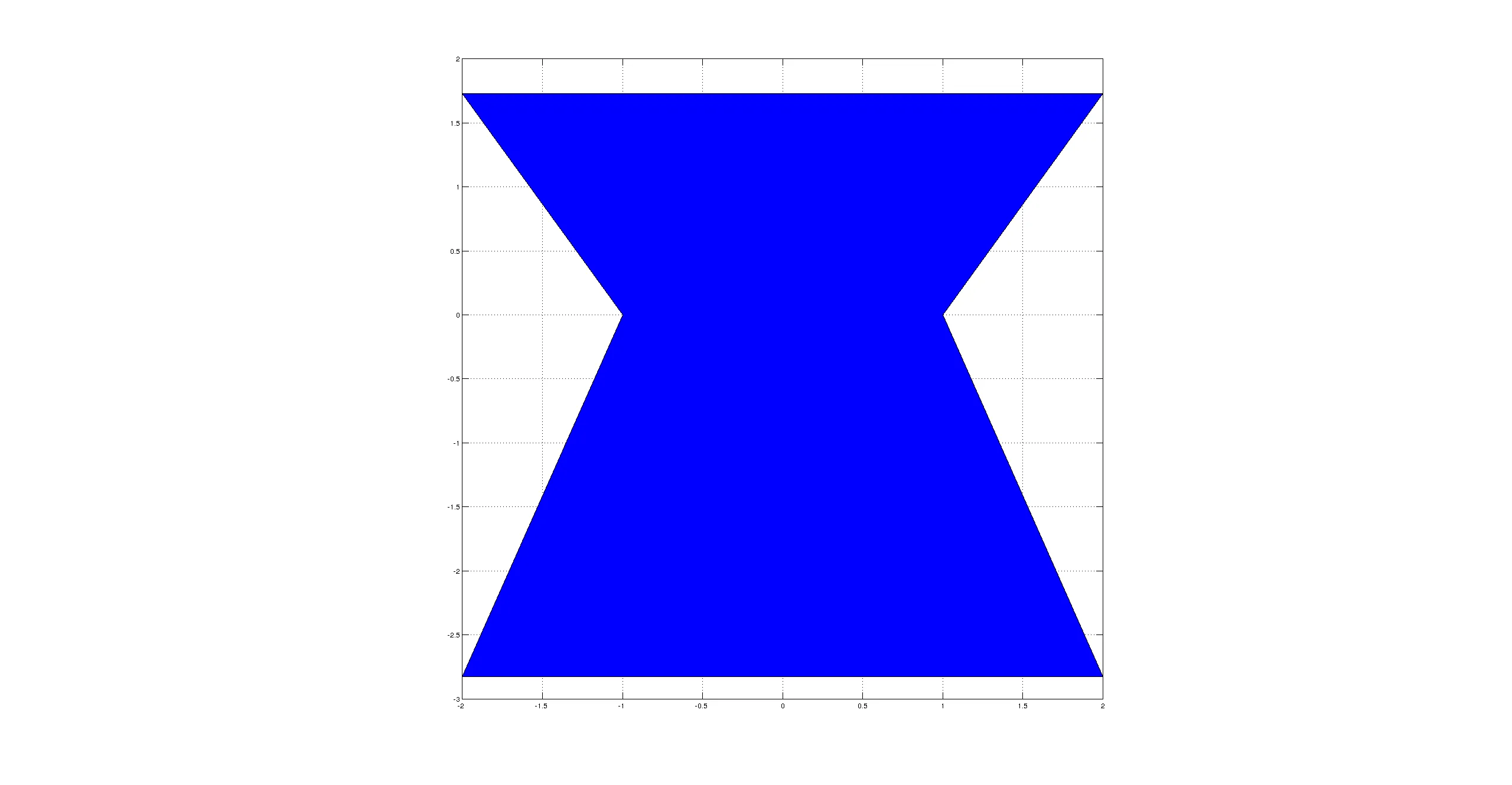
fill和fill3应该能够实现。以下是一个示例代码,假设您的六边形由两个宽度w1和w2以及d1和d2参数来参数化,它们是边的长度:function draw_hexagon(w1, w2, d1, d2)
a=(w1-w2)/2;
b1=sqrt(d1^2 - a^2);
b2=sqrt(d2^2 - a^2);
xs=[-w1/2, w1/2, w2/2, w1/2, -w1/2, -w2/2];
ys=[b1, b1, 0, -b2, -b2, 0];
fill(xs, ys, 'b')
axis square
grid on
end
它将为
w1=4, w2=2, d1=2, d2=3 生成以下内容:
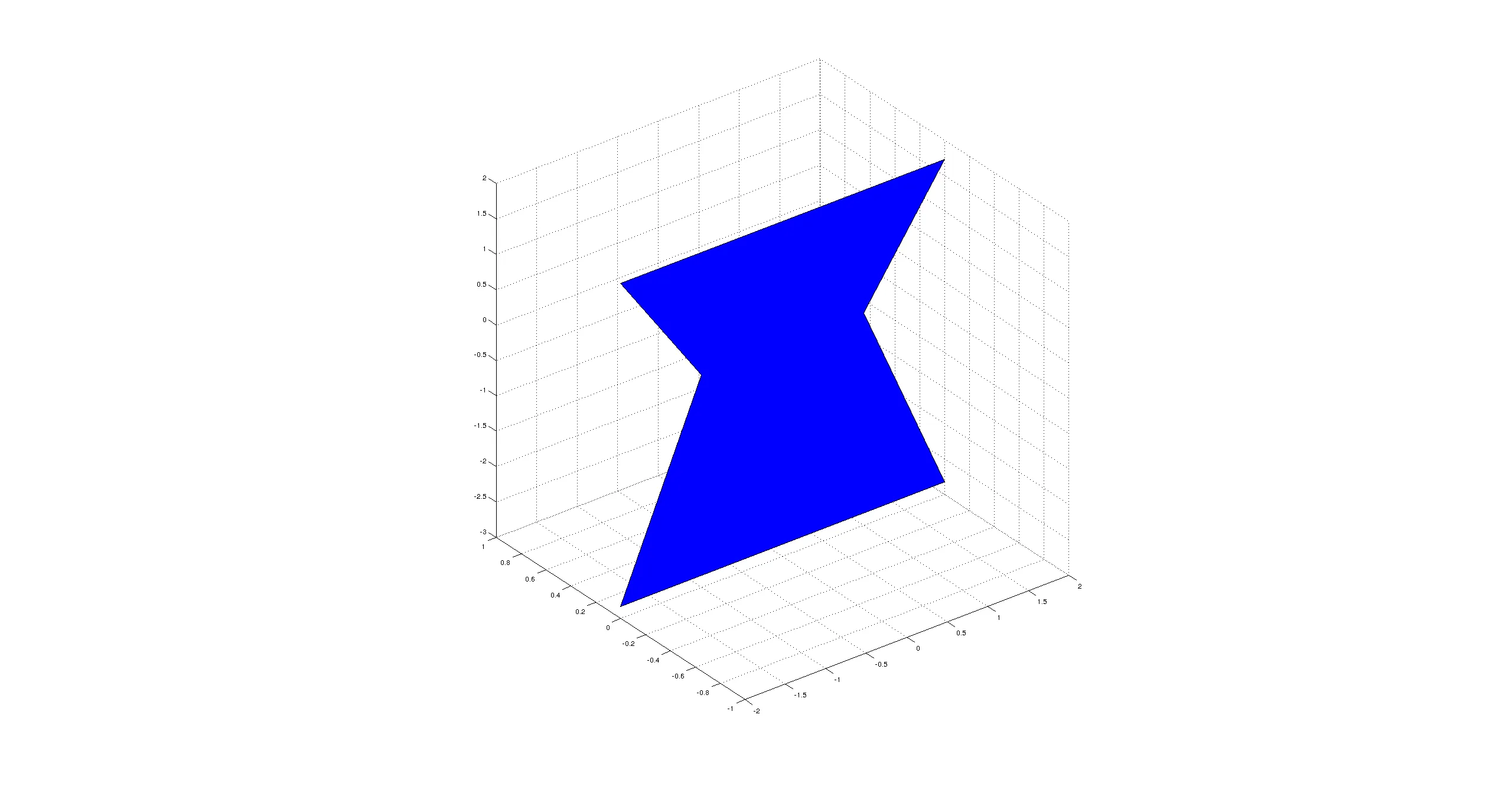
function draw_hexagon_3d(w1, w2, d1, d2)
    a=(w1-w2)/2;
    b1=sqrt(d1^2 - a^2);
    b2=sqrt(d2^2 - a^2);

    xs=[-w1/2, w1/2, w2/2, w1/2, -w1/2, -w2/2];
    ys=[0, 0, 0, 0, 0, 0];
    zs=[b1, b1, 0, -b2, -b2, 0];

    fill3(xs, ys, zs, 'b')
    grid on
    axis square
end
我们得到:
- Andrzej Pronobis
5
这又是一个很棒的答案!如此简单而优雅。正是我们在这里所需要的。我认为你的解决方案甚至比Bert的参数还要少,因为你没有直接的角度,但可以从你的参数中间接推导出来。 - Léo Léopold Hertz 준영
1我最初没有注意到d1和d2是边的长度。现在我已经在上面的代码中修正了这个问题,因此参数化是基于边缘的宽度和长度的。 - Andrzej Pronobis
不错的实现!这假设顶部和底部是平行的,并且六边形具有垂直对称轴。 - Bert
假设您不需要其他自由度,您可以按如下方式重新排列自由度。通过用它们的比率r1(和同样的r2)替换w1和d1,并将rw作为w1/r2添加,您可以完全定义形状并在独立参数中设置大小。 - Bert
我在下面添加了一篇维基页面,介绍如何通过语法最终构建网格。 - Léo Léopold Hertz 준영
1
尝试建立一个标准的网格库,我认为我们应该从确定自由度开始。对于具有2个口的凹面两侧对称六边形来说,它可能是:
- 口ax宽度(W_m)
- 相对顶部宽度(w_t = W_t / W_m)
- 相对底部宽度(w_b = W_b / W_m)
- 相对顶部高度
- 相对底部高度
- Bert
1
实际上,我认为你的答案比Margus和A_A更好地回答了这个问题。关键是要理解标准网格的标准化内容。非常好的想法! - Léo Léopold Hertz 준영
0
我和我的同事讨论了这个问题。 他建议创建一个三角形网络,但也指出了非凸多边形的一般算法。
使用自己的算法创建网格
- 通过虚线将六边形分成两个梯形,如问题描述中所示
- 将梯形分割成三角形:
assemmbly并通过inittri构建三角网结构 - 加载向量
f通过bilin_assembly构建(因为之前这样做过,但不一定是最优选择)
将具有两个口的六边形分成两个梯形
- 选择两个节点,其索引差为3且距离在六个节点中最小。
- 形成两个梯形,其中一个梯形包含数字1-4,而另一个包含数字1,6,5,4。
以下语法基于我在2013年对代码的修改,但主要参考了Claes Johnson的书《用有限元方法求解偏微分方程的数值解》的描述。
现在考虑汇编语言的语法,以简化泊松问题(稍后必须在此处进行精细处理)
% [S,f]=assemblyGlobal(loadfunction,mesh)
%
%   loadfunction = function on the right-hand side of the Poisson equation
%   mesh         = mesh structure on which the assembly is done
%
%   S            = stiffness matrix of the Poisson problem
%   f            = load vector corresponding to loadfunction
我们需要双线性汇编的语法在哪里
% function B=bilin_assembly(bilin,mesh)
%
%  bilin = function handle to integrand of the bilinear form
%          given as bilin(u,v,ux,uy,vx,vy,x,y), where
%          u  - values of function u
%          v  - values of function v
%          ux - x-derivative of function u
%          uy - y-derivative of function u
%          vx - x-derivative of function v
%          vy - y-derivative of function v
%          x  - global x-coordinate
%          y  - global y-coordinate
%  mesh  = mesh structure on which the matrix will be assembled
%
%  B     = matrix related to bilinear form bilin
初始化三角网格的语法
% function mesh = inittri(p,t)
%
%   p       = nodes
%   t       = triangles
%
%   mesh    = trimesh structure corresponding to (p,t)
%
% TRIMESH STRUCTURE :
%
%   p       = nodes in a 2xN-matrix
%
%   t       = triangles in a 3xN- matrix (nodes of the triangles as indeces to the p- matrix).
%
%   edges   = a matrix of all edges in the mesh. Each column is an edge :
%             [n1 ; n2] where n1 < n2;
%
%   t2e     = a matrix connecting  triangle's and edges's.
%             Each column corresponds to a triangle and has
%             triangle's edges in the order n1->n2, n2->n3,
%             n1->n3.
%
%   e2t     = inverse of t2e.
由于版权问题和答案会变得很长,我没有在这里发布完整的源代码。然而,所有算法都基于第一个源,因此任何研究人员都可以创建它们。我认为这种FEM方法是找到最佳网格的唯一途径。
用于一般非凸多边形的算法
还有一些算法可以为一般非凸多边形创建网格。Margus的答案提供的网格可能就是由这样的算法产生的。
Ansys
我正在尝试不同的产品来可视化孔洞、不同的几何形状和不同的材料。Ansys是一个有前途的解决方案。
来源
- 有限元方法求解偏微分方程的数值解,Claes Johnson著。
- 我大学2013-2014年度的有限元方法课堂笔记。
- Léo Léopold Hertz 준영
1
我不得不接受这个答案,因为它是唯一提供系统化查找标准网格的方法。如果有更好的答案能够提供免费源代码进行系统测试,我将非常乐意回答。 - Léo Léopold Hertz 준영
网页内容由stack overflow 提供, 点击上面的可以查看英文原文,
原文链接
原文链接