我怎样找到每个系数的p值(显著性)?
lm = sklearn.linear_model.LinearRegression()
lm.fit(x,y)
我怎样找到每个系数的p值(显著性)?
lm = sklearn.linear_model.LinearRegression()
lm.fit(x,y)
这有点过头了,但让我们试一下。首先使用statsmodel来找出p值应该是多少。
import pandas as pd
import numpy as np
from sklearn import datasets, linear_model
from sklearn.linear_model import LinearRegression
import statsmodels.api as sm
from scipy import stats

diabetes = datasets.load_diabetes()
X = diabetes.data
y = diabetes.target

X2 = sm.add_constant(X)
est = sm.OLS(y, X2)
est2 = est.fit()
print(est2.summary())
然后我们得到
                         OLS Regression Results
==============================================================================
Dep. Variable:                      y   R-squared:                       0.518
Model:                            OLS   Adj. R-squared:                  0.507
Method:                 Least Squares   F-statistic:                     46.27
Date:                Wed, 08 Mar 2017   Prob (F-statistic):           3.83e-62
Time:                        10:08:24   Log-Likelihood:                -2386.0
No. Observations:                 442   AIC:                             4794.
Df Residuals:                     431   BIC:                             4839.
Df Model:                          10
Covariance Type:            nonrobust
==============================================================================
                 coef    std err          t      P>|t|      [0.025      0.975]
------------------------------------------------------------------------------
const        152.1335      2.576     59.061      0.000     147.071     157.196
x1           -10.0122     59.749     -0.168      0.867    -127.448     107.424
x2          -239.8191     61.222     -3.917      0.000    -360.151    -119.488
x3           519.8398     66.534      7.813      0.000     389.069     650.610
x4           324.3904     65.422      4.958      0.000     195.805     452.976
x5          -792.1842    416.684     -1.901      0.058   -1611.169      26.801
x6           476.7458    339.035      1.406      0.160    -189.621    1143.113
x7           101.0446    212.533      0.475      0.635    -316.685     518.774
x8           177.0642    161.476      1.097      0.273    -140.313     494.442
x9           751.2793    171.902      4.370      0.000     413.409    1089.150
x10           67.6254     65.984      1.025      0.306     -62.065     197.316
==============================================================================
Omnibus:                        1.506   Durbin-Watson:                   2.029
Prob(Omnibus):                  0.471   Jarque-Bera (JB):                1.404
Skew:                           0.017   Prob(JB):                        0.496
Kurtosis:                       2.726   Cond. No.                         227.
==============================================================================
好的,让我们来复现这个过程。虽然使用矩阵代数来进行线性回归分析有点过头了,但没关系。
lm = LinearRegression()
lm.fit(X,y)
params = np.append(lm.intercept_,lm.coef_)
predictions = lm.predict(X)

newX = pd.DataFrame({"Constant":np.ones(len(X))}).join(pd.DataFrame(X))
MSE = (sum((y-predictions)**2))/(len(newX)-len(newX.columns))

# Note if you don't want to use a DataFrame replace the two lines above with
# newX = np.append(np.ones((len(X),1)), X, axis=1)
# MSE = (sum((y-predictions)**2))/(len(newX)-len(newX[0]))

var_b = MSE*(np.linalg.inv(np.dot(newX.T,newX)).diagonal())
sd_b = np.sqrt(var_b)
ts_b = params/ sd_b

p_values =[2*(1-stats.t.cdf(np.abs(i),(len(newX)-len(newX[0])))) for i in ts_b]

sd_b = np.round(sd_b,3)
ts_b = np.round(ts_b,3)
p_values = np.round(p_values,3)
params = np.round(params,4)

myDF3 = pd.DataFrame()
myDF3["Coefficients"],myDF3["Standard Errors"],myDF3["t values"],myDF3["Probabilities"] = [params,sd_b,ts_b,p_values]
print(myDF3)
    Coefficients  Standard Errors  t values  Probabilities
0       152.1335            2.576    59.061         0.000
1       -10.0122           59.749    -0.168         0.867
2      -239.8191           61.222    -3.917         0.000
3       519.8398           66.534     7.813         0.000
4       324.3904           65.422     4.958         0.000
5      -792.1842          416.684    -1.901         0.058
6       476.7458          339.035     1.406         0.160
7       101.0446          212.533     0.475         0.635
8       177.0642          161.476     1.097         0.273
9       751.2793          171.902     4.370         0.000
10       67.6254           65.984     1.025         0.306
因此,我们可以从statsmodel中重新生成这些值。
nan的问题。这是因为我的X是数据样本,所以索引出现了偏差。在调用pd.DataFrame.join()时会引发错误。我进行了一行修改,看起来现在可以工作了:newX = pd.DataFrame({"Constant":np.ones(len(X))}).join(pd.DataFrame(X.reset_index(drop=True)))。 - paultlen(newX)-len(X[0])而不是len(newX)-len(newX[0])。 - newbiescikit-learn的LinearRegression类不会计算这些信息,但您可以轻松扩展该类来实现:
from sklearn import linear_model
from scipy import stats
import numpy as np


class LinearRegression(linear_model.LinearRegression):
    """
    LinearRegression class after sklearn's, but calculate t-statistics
    and p-values for model coefficients (betas).
    Additional attributes available after .fit()
    are `t` and `p` which are of the shape (y.shape[1], X.shape[1])
    which is (n_features, n_coefs)
    This class sets the intercept to 0 by default, since usually we include it
    in X.
    """

    def __init__(self, *args, **kwargs):
        if not "fit_intercept" in kwargs:
            kwargs['fit_intercept'] = False
        super(LinearRegression, self)\
                .__init__(*args, **kwargs)

    def fit(self, X, y, n_jobs=1):
        self = super(LinearRegression, self).fit(X, y, n_jobs)

        sse = np.sum((self.predict(X) - y) ** 2, axis=0) / float(X.shape[0] - X.shape[1])
        se = np.array([
            np.sqrt(np.diagonal(sse[i] * np.linalg.inv(np.dot(X.T, X))))
                                                    for i in range(sse.shape[0])
                    ])

        self.t = self.coef_ / se
        self.p = 2 * (1 - stats.t.cdf(np.abs(self.t), y.shape[0] - X.shape[1]))
        return self
这里的内容来源于这里。
如果你想在Python中进行这种统计分析,你应该看看statsmodels。
import statsmodels.api as sm
mod = sm.OLS(Y,X)
fii = mod.fit()
p_values = fii.summary2().tables[1]['P>|t|']
elyase的回答中的代码https://dev59.com/0V4c5IYBdhLWcg3wa56M#27928411实际上并不起作用。请注意,sse是一个标量,然后它试图遍历它。以下代码是修改后的版本。不是非常干净,但我认为它基本上可以工作。
class LinearRegression(linear_model.LinearRegression):

    def __init__(self,*args,**kwargs):
        # *args is the list of arguments that might go into the LinearRegression object
        # that we don't know about and don't want to have to deal with. Similarly, **kwargs
        # is a dictionary of key words and values that might also need to go into the orginal
        # LinearRegression object. We put *args and **kwargs so that we don't have to look
        # these up and write them down explicitly here. Nice and easy.

        if not "fit_intercept" in kwargs:
            kwargs['fit_intercept'] = False

        super(LinearRegression,self).__init__(*args,**kwargs)

    # Adding in t-statistics for the coefficients.
    def fit(self,x,y):
        # This takes in numpy arrays (not matrices). Also assumes you are leaving out the column
        # of constants.

        # Not totally sure what 'super' does here and why you redefine self...
        self = super(LinearRegression, self).fit(x,y)
        n, k = x.shape
        yHat = np.matrix(self.predict(x)).T

        # Change X and Y into numpy matricies. x also has a column of ones added to it.
        x = np.hstack((np.ones((n,1)),np.matrix(x)))
        y = np.matrix(y).T

        # Degrees of freedom.
        df = float(n-k-1)

        # Sample variance.
        sse = np.sum(np.square(yHat - y),axis=0)
        self.sampleVariance = sse/df

        # Sample variance for x.
        self.sampleVarianceX = x.T*x

        # Covariance Matrix = [(s^2)(X'X)^-1]^0.5. (sqrtm = matrix square root.  ugly)
        self.covarianceMatrix = sc.linalg.sqrtm(self.sampleVariance[0,0]*self.sampleVarianceX.I)

        # Standard erros for the difference coefficients: the diagonal elements of the covariance matrix.
        self.se = self.covarianceMatrix.diagonal()[1:]

        # T statistic for each beta.
        self.betasTStat = np.zeros(len(self.se))
        for i in xrange(len(self.se)):
            self.betasTStat[i] = self.coef_[0,i]/self.se[i]

        # P-value for each beta. This is a two sided t-test, since the betas can be
        # positive or negative.
        self.betasPValue = 1 - t.cdf(abs(self.betasTStat),df)
您可以使用scipy计算p-value。以下代码来自scipy文档。
>>> from scipy import stats
>>> import numpy as np
>>> x = np.random.random(10)
>>> y = np.random.random(10)
>>> slope, intercept, r_value, p_value, std_err = stats.linregress(x,y)
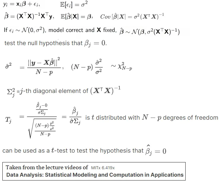
稍微了解一下线性回归的理论,以下是我们需要计算系数估计器(随机变量)的p值的总结,以检查它们是否显著(通过拒绝相应的零假设):
import numpy as np
# generate some data
np.random.seed(1)
n = 100
X = np.random.random((n,2))
beta = np.array([-1, 2])
noise = np.random.normal(loc=0, scale=2, size=n)
y = X@beta + noise
scikit-learn 计算上述公式的 p 值:# use scikit-learn's linear regression model to obtain the coefficient estimates
from sklearn.linear_model import LinearRegression
reg = LinearRegression().fit(X, y)
beta_hat = [reg.intercept_] + reg.coef_.tolist()
beta_hat
# [0.18444290873001834, -1.5879784718284842, 2.5252138207251904]
# compute the p-values
from scipy.stats import t
# add ones column
X1 = np.column_stack((np.ones(n), X))
# standard deviation of the noise.
sigma_hat = np.sqrt(np.sum(np.square(y - X1@beta_hat)) / (n - X1.shape[1]))
# estimate the covariance matrix for beta
beta_cov = np.linalg.inv(X1.T@X1)
# the t-test statistic for each variable from the formula from above figure
t_vals = beta_hat / (sigma_hat * np.sqrt(np.diagonal(beta_cov)))
# compute 2-sided p-values.
p_vals = t.sf(np.abs(t_vals), n-X1.shape[1])*2
t_vals
# array([ 0.37424023, -2.36373529, 3.57930174])
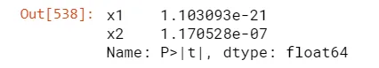
p_vals
# array([7.09042437e-01, 2.00854025e-02, 5.40073114e-04])
使用statsmodels计算p值:
import statsmodels.api as sm
X1 = sm.add_constant(X)
model = sm.OLS(y, X2)
model = model.fit()
model.tvalues
# array([ 0.37424023, -2.36373529,  3.57930174])
# compute p-values
t.sf(np.abs(model.tvalues), n-X1.shape[1])*2
# array([7.09042437e-01, 2.00854025e-02, 5.40073114e-04])

model.summary()
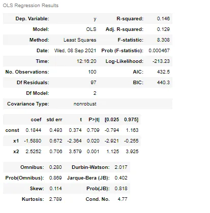
从上面可以看出,在这两种情况下计算得到的P值完全相同。
beta_cov中的一些对角元素为负,因此np.sqrt(np.diagonal(beta_cov))会失败,因为负数没有平方根。在这种情况下应该怎么做?你知道负值背后的原因吗? - Probhakar Sarkarimport pingouin as pg
# Using a Pandas DataFrame `df`:
lm = pg.linear_regression(df[['x', 'z']], df['y'])
# Using a NumPy array:
lm = pg.linear_regression(X, y)
输出是一个数据框,其中包括每个预测变量的 beta 系数、标准误差、T 值、p 值和置信区间,以及拟合的 R^2 和调整后的 R^2。
p_value是f统计量中的一个值。如果你想获取这个值,只需要使用下面几行代码:
import statsmodels.api as sm
from scipy import stats

diabetes = datasets.load_diabetes()
X = diabetes.data
y = diabetes.target

X2 = sm.add_constant(X)
est = sm.OLS(y, X2)
print(est.fit().f_pvalue)
除了已经提出的选项之外,另一个选择是使用排列测试。将值为y的模型进行N次拟合,并计算与原始模型给出的系数相比,拟合模型中具有更大值(单侧检验)或更大绝对值(双侧检验)的比例。这些比例就是p值。