当进行SVM-OVA时,我尝试绘制超平面,步骤如下:
import matplotlib.pyplot as plt
import numpy as np
from sklearn.svm import SVC
x = np.array([[1,1.1],[1,2],[2,1]])
y = np.array([0,100,250])
classifier = OneVsRestClassifier(SVC(kernel='linear'))
根据这个问题的答案 使用Python绘制线性SVM超平面, 我编写了以下代码:
fig, ax = plt.subplots()
# create a mesh to plot in
x_min, x_max = x[:, 0].min() - 1, x[:, 0].max() + 1
y_min, y_max = x[:, 1].min() - 1, x[:, 1].max() + 1
xx2, yy2 = np.meshgrid(np.arange(x_min, x_max, .2),np.arange(y_min, y_max, .2))
Z = classifier.predict(np.c_[xx2.ravel(), yy2.ravel()])
Z = Z.reshape(xx2.shape)
ax.contourf(xx2, yy2, Z, cmap=plt.cm.winter, alpha=0.3)
ax.scatter(x[:, 0], x[:, 1], c=y, cmap=plt.cm.winter, s=25)

# First line: class1 vs (class2 U class3)
w = classifier.coef_[0]
a = -w[0] / w[1]
xx = np.linspace(-5, 5)
yy = a * xx - (classifier.intercept_[0]) / w[1]
ax.plot(xx,yy)

# Second line: class2 vs (class1 U class3)
w = classifier.coef_[1]
a = -w[0] / w[1]
xx = np.linspace(-5, 5)
yy = a * xx - (classifier.intercept_[1]) / w[1]
ax.plot(xx,yy)

# Third line: class 3 vs (class2 U class1)
w = classifier.coef_[2]
a = -w[0] / w[1]
xx = np.linspace(-5, 5)
yy = a * xx - (classifier.intercept_[2]) / w[1]
ax.plot(xx,yy)
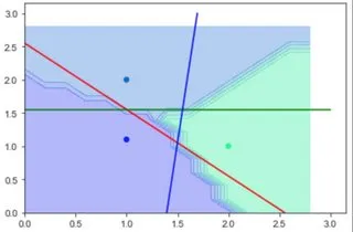
然而,这就是我所获得的:
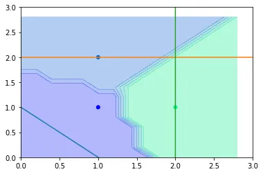
我画这些线条是错的吗?还是分类器由于训练点太少而无法正常工作?