司仪行走测试但之后保持不变

3
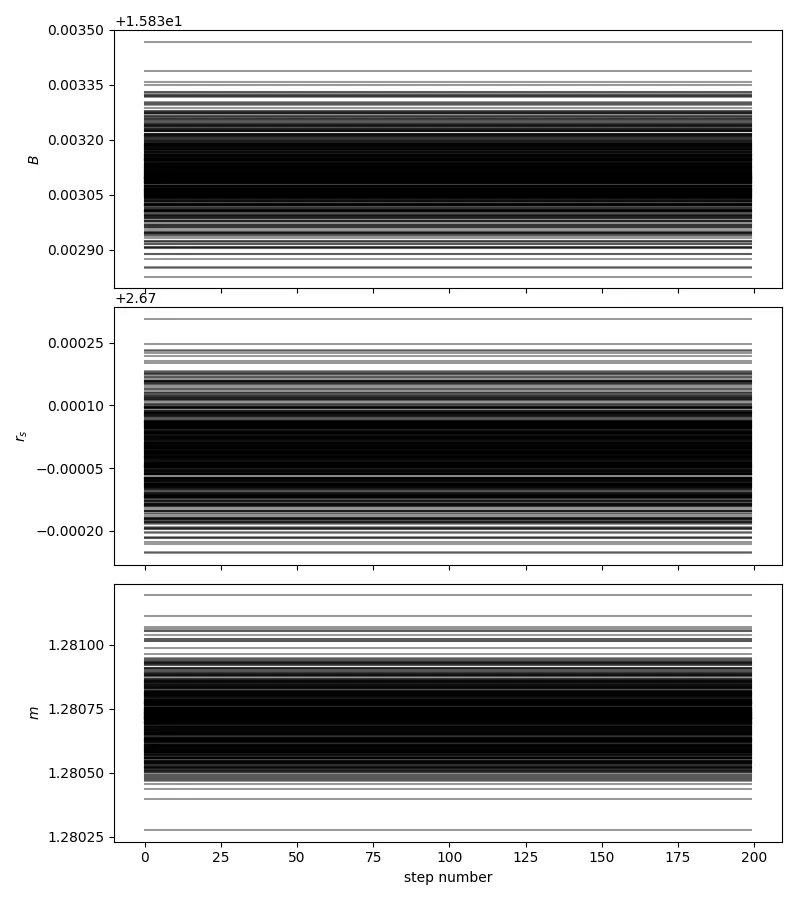
我使用emcee时遇到了问题。这是一个足够简单的三参数拟合,但偶尔(尽管经常使用,但迄今只发生在两种情况下)我的行走者刚开始很好地烧录,但是之后就不动了(见下图)。报告的接受率为0。
有其他人遇到过这个问题吗?我已经尝试改变我的初始条件、行走者数量和迭代次数等。这段代码在非常相似的数据集上运行良好。它并不是一个具有挑战性的参数空间,看起来行走者被“卡住”的可能性很小。
有什么想法吗?我被难住了...我的行走者似乎很懒...

enter image description here

以下是示例代码(和示例数据文件)。当我运行它时,这个代码和数据文件会失败。
`
import numpy as n
import math
import pylab as py    
import matplotlib.pyplot as plt
import scipy
from scipy.optimize import curve_fit
from scipy import ndimage
import pyfits
from scipy import stats
import emcee
import corner
import scipy.optimize as op
import matplotlib.pyplot as pl
from matplotlib.ticker import MaxNLocator

def sersic(x, B,r_s,m):
      return B * n.exp(-1.0 * (1.9992*m - 0.3271) * ( (x/r_s)**(1.0/m) - 1.))

def lnprior(theta):
      B,r_s,m, lnf = theta
      if  0.0 < B < 500.0 and 0.5 < m < 10. and r_s > 0. and -10.0 < lnf < 1.0: 
        return 0.0
      return -n.inf

def lnlike(theta, x, y, yerr): #"least squares"
      B,r_s,m, lnf = theta
      model = sersic(x,B, r_s, m)
      inv_sigma2 = 1.0/(yerr**2 + model**2*n.exp(2*lnf))
      return -0.5*(n.sum((y-model)**2*inv_sigma2 - n.log(inv_sigma2)))

def lnprob(theta, x, y, yerr):#kills based on priors
    lp = lnprior(theta)
    if not n.isfinite(lp):
        return -n.inf
    return lp + lnlike(theta, x, y, yerr)


profile=open("testprofile.dat",'r')  #read in the data file    
profilelines=profile.readlines()
x=n.empty(len(profilelines))
y=n.empty(len(profilelines))
yerr=n.empty(len(profilelines))

for i,line in enumerate(profilelines):
    col=line.split()
    x[i]=col[0]
    y[i]=col[1]
    yerr[i]=col[2]

# Find the maximum likelihood value.
chi2 = lambda *args: -2 * lnlike(*args)
result = op.minimize(chi2, [50,2.0,0.5,0.5], args=(x, y, yerr))
B_ml, rs_ml,m_ml, lnf_ml = result["x"]
print("""Maximum likelihood result:
          B   = {0}
          r_s = {1}
          m   = {2}
    """.format(B_ml, rs_ml,m_ml))

# Set up the sampler.
ndim, nwalkers = 4, 4000
pos = [result["x"] + 1e-4*n.random.randn(ndim) for i in     range(nwalkers)]
sampler = emcee.EnsembleSampler(nwalkers, ndim, lnprob, args=(x, y, yerr))
# Clear and run the production chain.
print("Running MCMC...")
Niter = 2000 #2000
sampler.run_mcmc(pos, Niter, rstate0=n.random.get_state())
print("Done.")
# Print out the mean acceptance fraction. 
af = sampler.acceptance_fraction
print "Mean acceptance fraction:", n.mean(af)

# Plot sampler chain
pl.clf()
fig, axes = pl.subplots(3, 1, sharex=True, figsize=(8, 9))
axes[0].plot(sampler.chain[:, :, 0].T, color="k", alpha=0.4)
axes[0].yaxis.set_major_locator(MaxNLocator(5))
axes[0].set_ylabel("$B$")

axes[1].plot(sampler.chain[:, :, 1].T, color="k", alpha=0.4)
axes[1].yaxis.set_major_locator(MaxNLocator(5))
axes[1].set_ylabel("$r_s$")

axes[2].plot(n.exp(sampler.chain[:, :, 2]).T, color="k", alpha=0.4)
axes[2].yaxis.set_major_locator(MaxNLocator(5))
axes[2].set_xlabel("step number")

fig.tight_layout(h_pad=0.0)
fig.savefig("line-time_test.png")

# plot MCMC fit
burnin = 100
samples = sampler.chain[:, burnin:, :3].reshape((-1, ndim-1))

B_mcmc, r_s_mcmc, m_mcmc = map(lambda v: (v[0]),
                         zip(*n.percentile(samples, [50],
                                            axis=0)))
print("""MCMC  result:
         B   = {0}
         r_s = {1}
         m   = {2}
    """.format(B_mcmc, r_s_mcmc, m_mcmc))

pl.close()

# Make the triangle plot.
burnin = 50
samples = sampler.chain[:, burnin:, :3].reshape((-1, ndim-1))

fig = corner.corner(samples, labels=["$B$", "$r_s$", "$m$"])
fig.savefig("line-triangle_test.png")

2
我们需要看到一个 [mcve]。这包括示例数据和可运行的代码,当在示例数据上运行时能够重现问题。如果我们看不到你正在运行什么,我们无法调试这个问题。 - user2357112
我已经添加了一个例子 - 它有点笨拙和冗长,但如果我简化一切,那么它就可以正常运行,没有问题... :( - astrohuman
1
你从卡方最小化(
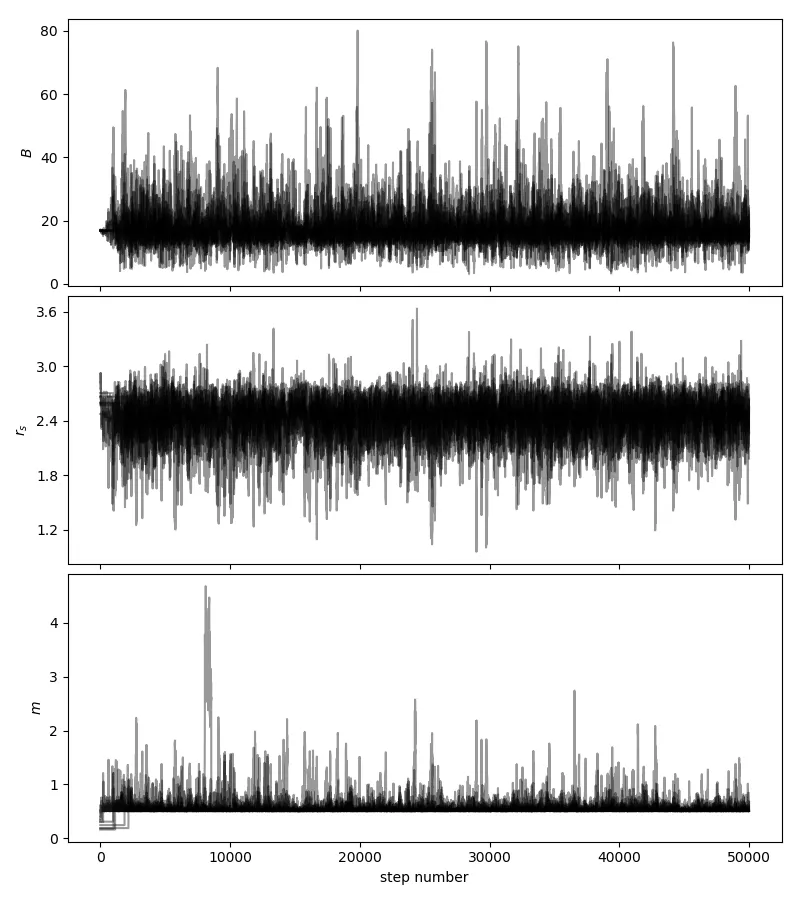
op.minimize)中得到了什么样的参数值?当我在你的示例上尝试时,返回的值非常大(以千计),这意味着初始行走者位置确实远离了你设定的先验边界。看看如果你只是让行走者从先验边界内均匀地随机选择一个起始点(或者在这些边界内的某个小球中),会发生什么情况。 - Matt Pitkin
3
你可能还想确保只保留有限概率的样本,例如 idx = n.isfinite(sampler.lnprobability[:,burnin:].reshape((Niter-burnin)*nwalkers)); newsamps = samples[idx,:],并通过计算每个参数的自相关时间来观察样本的稀疏化,例如 from emcee.autocorr import integrated_time; acls = []; for samps in newsamps.T: acls.append(integrated_time(samps)); newsamps = newsamps[0:-1:int(n.max(acls)),:] - Matt Pitkin
1个回答

1
这是一个更好的结果。我将随机初始样本设置得不那么接近最大似然值,并且使用较少的行走者/链条运行了更多的步骤。请注意,我绘制的是参数m而不是它的指数,就像你所做的那样。
平均接受率约为0.48,我的笔记本电脑运行时间约为1分钟。当然,您可以添加更多的步骤并获得更好的结果。

enter image description here

import numpy as n
import emcee
import corner
import scipy.optimize as op
import matplotlib.pyplot as pl
from matplotlib.ticker import MaxNLocator


def sersic(x, B, r_s, m):
    return B * n.exp(
        -1.0 * (1.9992 * m - 0.3271) * ((x / r_s)**(1.0 / m) - 1.))


def lnprior(theta):
    B, r_s, m, lnf = theta
    if 0.0 < B < 500.0 and 0.5 < m < 10. and r_s > 0. and -10.0 < lnf < 1.0:
        return 0.0
    return -n.inf


def lnlike(theta, x, y, yerr):  # "least squares"
    B, r_s, m, lnf = theta
    model = sersic(x, B, r_s, m)
    inv_sigma2 = 1.0 / (yerr**2 + model**2 * n.exp(2 * lnf))
    return -0.5 * (n.sum((y - model)**2 * inv_sigma2 - n.log(inv_sigma2)))


def lnprob(theta, x, y, yerr):  # kills based on priors
    lp = lnprior(theta)
    if not n.isfinite(lp):
        return -n.inf
    return lp + lnlike(theta, x, y, yerr)


profile = open("testprofile.dat", 'r')  # read in the data file
profilelines = profile.readlines()
x = n.empty(len(profilelines))
y = n.empty(len(profilelines))
yerr = n.empty(len(profilelines))

for i, line in enumerate(profilelines):
    col = line.split()
    x[i] = col[0]
    y[i] = col[1]
    yerr[i] = col[2]

# Find the maximum likelihood value.
chi2 = lambda *args: -2 * lnlike(*args)
result = op.minimize(chi2, [50, 2.0, 0.5, 0.5], args=(x, y, yerr))
B_ml, rs_ml, m_ml, lnf_ml = result["x"]
print("""Maximum likelihood result:
          B   = {0}
          r_s = {1}
          m   = {2}
          lnf = {3}
    """.format(B_ml, rs_ml, m_ml, lnf_ml))

# Set up the sampler.
ndim, nwalkers = 4, 10
pos = [result["x"] + 1e-1 * n.random.randn(ndim) for i in range(nwalkers)]

sampler = emcee.EnsembleSampler(nwalkers, ndim, lnprob, args=(x, y, yerr))
# Clear and run the production chain.
print("Running MCMC...")
Niter = 50000
sampler.run_mcmc(pos, Niter, rstate0=n.random.get_state())
print("Done.")
# Print out the mean acceptance fraction.
af = sampler.acceptance_fraction
print("Mean acceptance fraction:", n.mean(af))

# Plot sampler chain
pl.clf()
fig, axes = pl.subplots(3, 1, sharex=True, figsize=(8, 9))
axes[0].plot(sampler.chain[:, :, 0].T, color="k", alpha=0.4)
axes[0].yaxis.set_major_locator(MaxNLocator(5))
axes[0].set_ylabel("$B$")

axes[1].plot(sampler.chain[:, :, 1].T, color="k", alpha=0.4)
axes[1].yaxis.set_major_locator(MaxNLocator(5))
axes[1].set_ylabel("$r_s$")

# axes[2].plot(n.exp(sampler.chain[:, :, 2]).T, color="k", alpha=0.4)
axes[2].plot(sampler.chain[:, :, 2].T, color="k", alpha=0.4)
axes[2].yaxis.set_major_locator(MaxNLocator(5))
axes[2].set_ylabel("$m$")
axes[2].set_xlabel("step number")

fig.tight_layout(h_pad=0.0)
fig.savefig("line-time_test.png")

# plot MCMC fit
burnin = 10000
samples = sampler.chain[:, burnin:, :3].reshape((-1, ndim - 1))

B_mcmc, r_s_mcmc, m_mcmc = map(
    lambda v: (v[0]), zip(*n.percentile(samples, [50], axis=0)))
print("""MCMC  result:
         B   = {0}
         r_s = {1}
         m   = {2}
    """.format(B_mcmc, r_s_mcmc, m_mcmc))

pl.close()

# Make the triangle plot.
burnin = 50
samples = sampler.chain[:, burnin:, :3].reshape((-1, ndim - 1))

fig = corner.corner(samples, labels=["$B$", "$r_s$", "$m$"])
fig.savefig("line-triangle_test.png")

网页内容由stack overflow 提供, 点击上面的
可以查看英文原文,
原文链接