ggplot2 - 在循环中使用scale_fill_manual无法应用颜色

Question

我正在运行一个循环，以获取数据集的每个子设置下的地图，并相应地应用给定的调色板（和相应的图例）。

人们倾向于不喜欢使用for()循环，并最大化其方法的向量化。我不知道如何将这个特定数据集的过程向量化。

在这种情况下，我处理一个相对较大的数据集（分布物种图集），这个数据集特别复杂，因为使用了不同的方法，并且必须为每个物种传递不同的选项，考虑到特定季节、不同的观察集等。 物种可能存在于一个季节中，而在另一个季节中则不会出现（它们可能是繁殖者、居民或迁移者）。应该为所有情况（季节）创建地图，在不存在时为空。除了现场工作之外，还可以使用其他数据。 地图图例必须适应所有变化，除了以自定义离散比例呈现感兴趣的变量（丰度）。

通过运行循环，我感到（根据我的有限专业知识）我可以更容易地保留和控制需要的几个对象，同时步入我创建的流中以产生所需的部分，并最终创建物种分布地图集。

我的问题是，我将每个结果的ggplot存储在一个list()对象中。每个季节的每个物种都将存储在一个列表中。我面临的问题与scale_fill_manual有关，当它在循环内部使用时会出现问题。行为很奇怪，因为我完成了地图，但颜色仅应用于最后一个ggplot输出。尽管如此，所有值仍然在图例中正确识别。

举个例子：

软件包

if (!require(ggplot2)) install.packages("ggplot2",
    repos = "http://cran.r-project.org"); library(ggplot2)
if (!require(grid)) install.packages("grid",
    repos = "http://cran.r-project.org"); library(grid)
if (!require(RColorBrewer)) install.packages("RColorBrewer",
    repos = "http://cran.r-project.org"); library(RColorBrewer)
if (!require(reshape)) install.packages("reshape",
    repos = "http://cran.r-project.org"); library(reshape)

首先是一个简单的例子

#Create a list of colors to be used with scale_manual
palette.l <- list()
palette.l[[1]] <- c('red', 'blue', 'green')
palette.l[[2]] <- c('pink', 'blue', 'yellow')
# Store each ggplot in a list object
plot.l <- list()
#Loop it
for(i in 1:2){
  plot.l[[i]] <- qplot(mpg, wt, data = mtcars, colour = factor(cyl)) +
    scale_colour_manual(values = palette.l[[i]])
}

在我的绘图会话中，plot.l[1] 将使用来自 palette.l[2] 的颜色进行绘制。

我的特定情况

函数

排列图表

ArrangeGraph <- function(..., nrow=NULL, ncol=NULL, as.table=FALSE) {
  dots <- list(...)
  n <- length(dots)
  if(is.null(nrow) & is.null(ncol)) { nrow = floor(n/2) ; ncol = ceiling(n/nrow)}
  if(is.null(nrow)) { nrow = ceiling(n/ncol)}
  if(is.null(ncol)) { ncol = ceiling(n/nrow)}
  ## NOTE see n2mfrow in grDevices for possible alternative
  grid.newpage()
  pushViewport(viewport(layout=grid.layout(nrow,ncol)))
  ii.p <- 1
  for(ii.row in seq(1, nrow)) {
    ii.table.row <- ii.row
    if(as.table) {ii.table.row <- nrow - ii.table.row + 1}
    for(ii.col in seq(1, ncol)) {
      ii.table <- ii.p
      if(ii.p > n) break
      print(dots[[ii.table]], vp=VPortLayout(ii.table.row, ii.col))
      ii.p <- ii.p + 1
    }
  }
}

视口

VPortLayout <- function(x, y) viewport(layout.pos.row=x, layout.pos.col=y)

物种数据集

bd.aves.1 <- structure(list(quad = c("K113", "K114", "K114", "K114", "K114",...
due to limited body character number limit, please download entire code from
https://docs.google.com/open?id=0BxSZDr4eTnb9R09iSndzZjBMS28

物种清单

list.esp.1 <- c("Sylv mela", "Saxi rube","Ocea leuc")#
# download from the above link

一些分类和其他数据

txcon.1 <- structure(list(id = c(156L, 359L, 387L), grupo = c("Aves", "Aves",# 
# download from the above link

季节

kSeason.1 <- c("Inverno", "Primavera", "Outono")

一个示例网格

grid500.df.1 <- structure(list(id = c("K113", "K113", "K113", "K113", "K113",#... 
# download from the above link

额外的映射元素

海岸线

coastline.df.1 <- structure(list(long = c(182554.963670234, 180518, 178865.39,#...
# download from the above link

标签位置调整

kFacx1 <- c(9000, -13000, -10000, -12000)

R 代码

for(i in listsp.1) { # LOOP 1 - Species
  # Set up objects 
  sist.i <- list() # Sistematic observations
  nsist.i <- list() # Non-Sistematic observations
  breaks.nind.1 <- list() # Breaks on abundances
  ## Grid and merged dataframe
  spij.1 <- list() # Stores a dataframe for sp i at season j
  ## Palette build
  classes.1 <- list()
  cllevels.1 <- list()
  palette.nind.1 <- list() # Color palette
  ## Maps
  grid500ij.1 <- list() # Grid for species i at season j
  map.dist.ij.1 <- NULL
  for(j in 1:length(kSeason.1)) { # LOOP 2 - Seasons
    # j assume each season: Inverno, Primavera, Outono
    # Sistematic occurences ===================================================
    sist.i.tmp <- nrow(subset(bd.aves.1, esp == i & cod_tipo %in% sistematica &
      periodo == kSeason.1[j]))
    if (sist.i.tmp!= 0) { # There is sistematic entries, Then:
      sist.i[[j]]<- ddply(subset(bd.aves.1,
                                 esp == i & cod_tipo %in% sistematica & 
                                   periodo == kSeason.1[j]),
                          .(periodo, quad), summarise, nind = sum(n_ind),
                          codnid = max(cod_nidi))
    } else { # No Sistematic entries, Then: 
      sist.i[[j]] <- data.frame('quad' = NA, 'periodo' = NA, 'nind' = NA, 
                                'codnid' = NA, stringsAsFactors = F)
    }
    # Additional Entries (RS1) e other non-sistematic entries  (biblio) =======
    nsist.tmp.i = nrow(subset(bd.aves.1, esp == i & !cod_tipo %in% sistematica &
      periodo == kSeason.1[j]))
    if (nsist.tmp.i != 0) { # RS1 and biblio entries, Then:
      nsist.i[[j]] <- subset(bd.aves.1,
                             esp == i & !cod_tipo %in% sistematica &
                               periodo == kSeason.1[j] & 
                               !quad %in% if (nrow(sist.i[[j]]) != 0) {
                                            subset(sist.i[[j]],
                                                   select = quad)$quad
                                          } else NA,
                             select = c(quad, periodo, cod_tipo, cod_nidi)
                             )
      names(nsist.i[[j]])[4] <- 'codnid'
    } else { # No RS1 and biblio entries, Then:      
        nsist.i[[j]] = data.frame('quad' = NA, 'periodo' = NA, 'cod_tipo' = NA,
                                'codnid' = NA, stringsAsFactors = F)
      }
    # Quantile breaks =========================================================
    if (!is.na(sist.i[[j]]$nind[1])) {
      breaks.nind.1[[j]] <- c(0,
                            unique(
                              ceiling(
                                quantile(unique(
                                  subset(sist.i[[j]], is.na(nind) == F)$nind), 
                                         q = seq(0, 1, by = 0.25)))))
    } else {
        breaks.nind.1[[j]] <- 0
      }
    # =========================================================================
    # Build Species dataframe and merge to grid
    # =========================================================================
    if (!is.na(sist.i[[j]]$nind[1])) { # There are Sistematic entries, Then:
      spij.1[[j]] <- merge(unique(subset(grid500df.1, select = id)),
                         sist.i[[j]],
                         by.x = 'id', by.y = 'quad', all.x = T)
      # Adjust abundances when equals to NA ===================================
      spij.1[[j]]$nind[is.na(spij.1[[j]]$nind) == T] <- 0
      # Break abundances to create discrete variable ==========================
      spij.1[[j]]$cln <- if (length(breaks.nind.1[[j]]) > 2) {
        cut(spij.1[[j]]$nind, breaks = breaks.nind.1[[j]], 
            include.lowest = T, right = F)
        } else {
            cut2(spij.1[[j]]$nind, g = 2)
          }
      # Variable Abundance ====================================================
      classes.1[[j]] = nlevels(spij.1[[j]]$cln)
      cllevels.1[[j]] = levels(spij.1[[j]]$cln)
      # Color Palette for abundances - isolated Zero class (color #FFFFFF) ====
      if (length(breaks.nind.1[[j]]) > 2) {
        palette.nind.1[[paste(kSeason.1[j])]] = c("#FFFFFF", brewer.pal(length(
          cllevels.1[[j]]) - 1, "YlOrRd"))
      } else {
          palette.nind.1[[paste(kSeason.1[j])]] = c(
            "#FFFFFF",  brewer.pal(3, "YlOrRd"))[1:classes.1[[j]]]
        }
        names(palette.nind.1[[paste(kSeason.1[j])]])[1 : length(
          palette.nind.1[[paste(kSeason.1[j])]])] <- cllevels.1[[j]]
      # Add RS1 and bilbio values to palette ==================================
      palette.nind.1[[paste(kSeason.1[j])]][length(
        palette.nind.1[[paste(kSeason.1[j])]]) + 1] <- '#CCC5AF'
      names(palette.nind.1[[paste(kSeason.1[j])]])[length(
        palette.nind.1[[paste(kSeason.1[j])]])] <- 'Suplementar'
      palette.nind.1[[paste(kSeason.1[j])]][length(
        palette.nind.1[[paste(kSeason.1[j])]]) + 1] <- '#ADCCD7'
      names(palette.nind.1[[paste(kSeason.1[j])]])[length(
        palette.nind.1[[paste(kSeason.1[j])]])] <- 'Bibliografia'
      # Merge species i dataframe to grid map =================================
      grid500ij.1[[j]] <- subset(grid500df.1, select = c(id, long, lat, order))
      grid500ij.1[[j]]$cln = merge(grid500ij.1[[j]],
                                 spij.1[[j]],
                                 by.x = 'id', by.y = 'id', all.x = T)$cln
      # Adjust factor levels of cln variable - Non-Sistematic data ============
      levels(grid500ij.1[[j]]$cln) <- c(levels(grid500ij.1[[j]]$cln), 'Suplementar',
                                      'Bibliografia')
      if (!is.na(nsist.i[[j]]$quad[1])) {
        grid500ij.1[[j]]$cln[grid500ij.1[[j]]$id %in% subset(
          nsist.i[[j]], cod_tipo == 'RS1', select = quad)$quad] <- 'Suplementar'
        grid500ij.1[[j]]$cln[grid500ij.1[[j]]$id %in% subset(
          nsist.i[[j]], cod_tipo == 'biblio', select = quad)$quad] <- 'Bibliografia'
      }
    } else { # No Sistematic entries, Then:
        if (!is.na(nsist.i[[j]]$quad[1])) { # RS1 or Biblio entries, Then:
          grid500ij.1[[j]] <- grid500df
          grid500ij.1[[j]]$cln <- '0'
          grid500ij.1[[j]]$cln <- factor(grid500ij.1[[j]]$cln)
          levels(grid500ij.1[[j]]$cln) <- c(levels(grid500ij.1[[j]]$cln),
                                          'Suplementar', 'Bibliografia')
          grid500ij.1[[j]]$cln[grid500ij.1[[j]]$id %in% subset(
            nsist.i[[j]], cod_tipo == 'RS1', 
            select = quad)$quad] <- 'Suplementar'
          grid500ij.1[[j]]$cln[grid500ij.1[[j]]$id %in% subset(
            nsist.i[[j]],cod_tipo == 'biblio', 
            select = quad)$quad] <- 'Bibliografia'
        } else { # No entries, Then:
            grid500ij.1[[j]] <- grid500df
            grid500ij.1[[j]]$cln <- '0' 
            grid500ij.1[[j]]$cln <- factor(grid500ij.1[[j]]$cln)
            levels(grid500ij.1[[j]]$cln) <- c(levels(grid500ij.1[[j]]$cln),
                                            'Suplementar', 'Bibliografia')      
          }
      } # End of Species dataframe build
    # Distribution Map for  species i at season j =============================    
    if (!is.na(sist.i[[j]]$nind[1])) { # There is sistematic entries, Then:
      map.dist.ij.1[[paste(kSeason.1[j])]] <- ggplot(grid500ij.1[[j]],
                                                  aes(x = long, y = lat)) +
        geom_polygon(aes(group = id, fill = cln), colour = 'grey80') +
        coord_equal() +
        scale_x_continuous(limits = c(100000, 180000)) +
        scale_y_continuous(limits = c(-4000, 50000)) +
        scale_fill_manual(
          name = paste("LEGEND",
                       '\nSeason: ', kSeason.1[j],
                       '\n% of Occupied Cells : ',
                         sprintf("%.1f%%", (length(unique(
                           grid500ij.1[[j]]$id[grid500ij.1[[j]]$cln != levels(
                           grid500ij.1[[j]]$cln)[1]]))/12)*100), # percent 
                        sep = ""
                       ),
          # Set Limits
          limits = names(palette.nind.1[[j]])[2:length(names(palette.nind.1[[j]]))],
          values = palette.nind.1[[j]][2:length(names(palette.nind.1[[j]]))],
          drop = F) +
          opts(
            panel.background = theme_rect(),
            panel.grid.major = theme_blank(),
            panel.grid.minor = theme_blank(),
            axis.ticks = theme_blank(),
            title = txcon.1$especie[txcon.1$esp == i],
            plot.title = theme_text(size = 10, face = 'italic'),
            axis.text.x = theme_blank(),
            axis.text.y = theme_blank(),
            axis.title.x = theme_blank(),
            axis.title.y = theme_blank(),
            legend.title = theme_text(hjust = 0,size = 10.5),
            legend.text = theme_text(hjust = -0.2, size = 10.5)
          ) +
          # Shoreline
          geom_path(inherit.aes = F, aes(x = long, y = lat),
                    data = coastline.df.1, colour = "#997744") +
          # Add localities
          geom_point(inherit.aes = F, aes(x = x, y = y),  colour = 'grey20',
                     data = localidades, size = 2) +
          # Add labels
          geom_text(inherit.aes = F, aes(x = x, y = y, label = c('Burgau',
                                                                 'Sagres')),
                    colour = "black",
                    data = data.frame(x = c(142817 + kFacx1[1], 127337 + kFacx1[4]),
                                      y = c(11886, 3962), size = 3))
    } else { # NO sistematic entries,then:
        map.dist.ij.1[[paste(kSeason.1[j])]] <- ggplot(grid500ij.1[[j]],
                                                    aes(x = long, y = lat)) +
          geom_polygon(aes.inherit = F, aes(group = id, fill = cln),
                       colour = 'grey80') +
          #scale_color_manual(values = kCorLimiteGrid) +
          coord_equal() +
          scale_x_continuous(limits = c(100000, 40000)) +
          scale_y_continuous(limits = c(-4000, 180000)) +
          scale_fill_manual(
            name = paste('LEGENDA',
                         '\nSeason: ', kSeason.1[j],
                         '\n% of Occupied Cells :',
                         sprintf("%.1f%%", (length(unique(
                           grid500ij.1[[j]]$id[grid500ij.1[[j]]$cln != levels(
                           grid500ij.1[[j]]$cln)[1]]))/12 * 100)), # percent 
                         sep = ''),
            limits = names(kPaletaNsis)[2:length(names(kPaletaNsis))],
            values = kPaletaNsis[2:length(names(kPaletaNsis))],
            drop = F) +
            opts(
              panel.background = theme_rect(),
              panel.grid.major = theme_blank(),
              panel.grid.minor = theme_blank(),
              title = txcon.1$especie[txcon.1$esp == i],
              plot.title = theme_text(size = 10, face = 'italic'),
              axis.ticks = theme_blank(),
              axis.text.x = theme_blank(),
              axis.text.y = theme_blank(),
              axis.title.x = theme_blank(),
              axis.title.y = theme_blank(),
              legend.title = theme_text(hjust = 0,size = 10.5),
              legend.text = theme_text(hjust = -0.2, size = 10.5)
            ) +
            # Add Shoreline
            geom_path(inherit.aes = F, data = coastline.df.1,
                      aes(x = long, y = lat),
                      colour = "#997744") +
            # Add Localities
            geom_point(inherit.aes = F, aes(x = x, y = y),
                       colour = 'grey20',
                       data = localidades, size = 2) +
            # Add labels
            geom_text(inherit.aes = F, aes(x = x, y = y,
                                           label = c('Burgau', 'Sagres')),
                      colour = "black",
                      data = data.frame(x = c(142817 + kFacx1[1],
                                              127337 + kFacx1[4],),
                                        y = c(11886, 3962)),
                      size = 3)
      } # End of Distribution map building for esp i and j seasons
  } # Fim do LOOP 2: j Estacoes
  # Print Maps
  png(file = paste('panel_species',i,'.png', sep = ''), res = 96, 
      width = 800, height = 800)
  ArrangeGraph(map.dist.ij.1[[paste(kSeason.1[3])]],
               map.dist.ij.1[[paste(kSeason.1[2])]],
               map.dist.ij.1[[paste(kSeason.1[1])]],
               ncol = 2, nrow = 2)
  dev.off()
  graphics.off()
} # End of LOOP 1

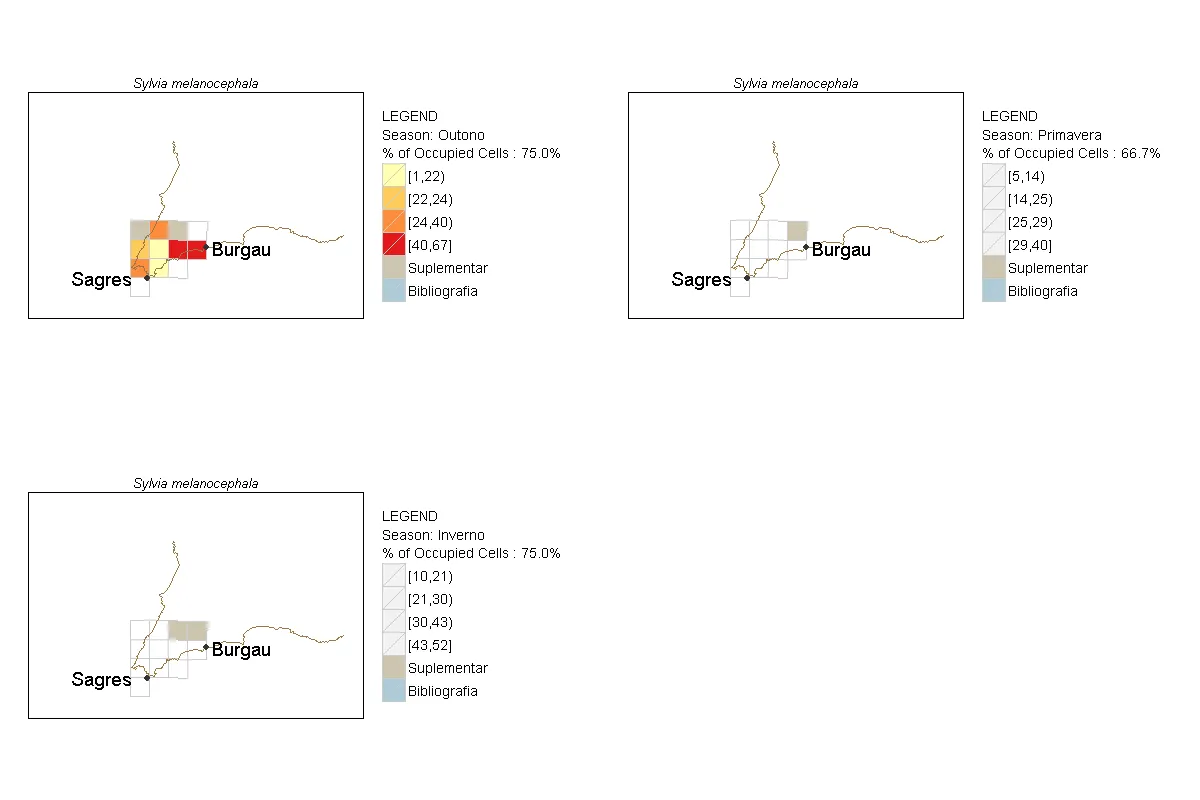
map.dist.ij.1[[paste(kSeason.1[3])]]是唯一一个应用于多边形的调色板，但每个j地图的图例项都很清晰定义。

R代码输出

正如我们所看到的，传奇很好，但是没有上色。 希望没有漏掉任何东西。对于一些缺失的葡萄牙术语请见谅。

- Paulo E. Cardoso

---

我建议使用两个循环，一个用于数据处理，另一个用于绘图。这样可以更轻松地调试代码。 - Luciano Selzer

相关的是，对于那些可能想要提供帮助的人来说，需要筛选大量的代码。您似乎在使用 fill 美学时遇到了一些问题。尝试构建一个最小可能的示例以说明您的问题将对您和愿意提供帮助的人都非常有帮助。 - joran

@lselzer。我同意代码很长，一开始可能看起来很难弄清楚事情是如何完成的。 - Paulo E. Cardoso

你的代码中“R代码”部分第一行有错别字吗？它目前写成了for(i in listsp.1)，但看起来应该是for(i in list.esp.1)。不过我不能确定——我还没有能够在我的系统上安装所有的包来测试你的代码。 - A5C1D2H2I1M1N2O1R2T1

这是我迄今为止没有阅读过的最长的帖子！ - Arun

Answer 1

老实说，我还没有仔细研究你的代码来解决你的具体问题——有点太多需要浏览了！但是对于你的演示例子，可以在循环中添加print(plot.l[[i]])。

#Create a list of colors to be used with scale_manual
palette.l <- list()
palette.l[[1]] <- c('red', 'blue', 'green')
palette.l[[2]] <- c('pink', 'blue', 'yellow')

# Store each ggplot in a list object
plot.l <- list()

# Loop it
for(i in 1:2) {
  plot.l[[i]] <- qplot(mpg, wt, data = mtcars, colour = factor(cyl)) +
    scale_colour_manual(values = palette.l[[i]])
  print(plot.l[[i]]) ### Added to your loop
}

---

在您的最小示例中，这也可以工作（无需先创建一个空列表来存储您的绘图），我认为它至少看起来更加简洁。我不确定是否可以将类似的方法适应于您的更大场景。

#Create a list of colors to be used with scale_manual
palette.l <- list(c('red', 'blue', 'green'),
                  c('pink', 'blue', 'yellow'))

p <- qplot(mpg, wt, data = mtcars, colour = factor(cyl))

# Use lapply and "force" to get your plots in a list    
plot.l <- lapply(palette.l, 
                 function(x) { 
                   force(x)
                   p + scale_color_manual(values = x) 
                 })

- A5C1D2H2I1M1N2O1R2T1