PyTorch中的.view()是什么意思？

Question

PyTorch中的.view()是什么意思？

337

.view() 方法对一个张量 x 做什么？负数值代表什么意思？

x = x.view(-1, 16 * 5 * 5)

- Wasi Ahmad

9个回答

63

view()函数通过“拉伸”或“压缩”张量的元素来将其重塑为您指定的形状：

`view()`如何工作？

首先，让我们看看张量在底层是什么：


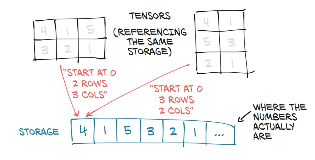
张量及其基础`storage`	例如，可以使用`t2 = t1.view(3,2)`从左张量（形状为（3,2））计算出右侧张量。

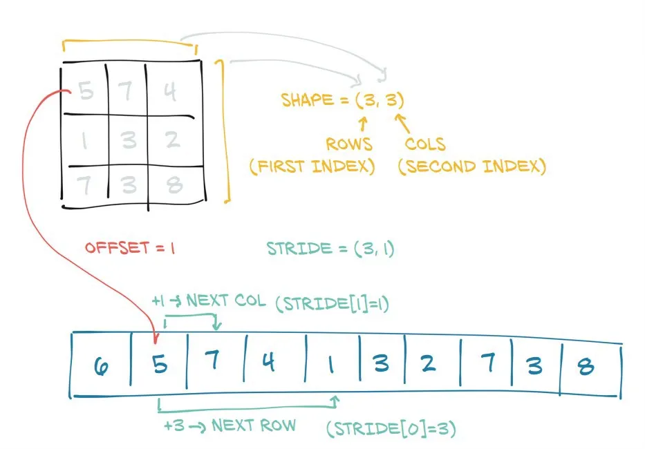
在这里，您可以看到PyTorch通过添加shape和stride属性，将连续内存块转换为类似于矩阵的对象来创建张量：

shape表示每个维度的长度
stride表示在每个维度中到达下一个元素需要在内存中走过多少步

view(dim1, dim2, ...) 返回一个相同底层信息的视图，但是将其重塑为形状为dim1 x dim2 x ...的张量(通过修改shape和stride属性)。

请注意，这暗示着新旧维度具有相同的乘积(即原始张量和新张量具有相同的体积)。

PyTorch -1

-1 是 PyTorch 中的别名，表示“推断给定其他维度都已指定的情况下该维度”的值(即原始乘积除以新乘积的商)。它是从numpy.reshape()采用的约定。

因此，在我们的例子中，t1.view(3,2)等价于t1.view(3,-1)或t1.view(-1,2)。

- iacob

56

让我们做一些例子，从简单到困难。

view 方法返回一个张量，其数据与 self 张量相同（这意味着返回的张量具有相同数量的元素），但形状不同。例如：

a = torch.arange(1, 17)  # a's shape is (16,)

a.view(4, 4) # output below
  1   2   3   4
  5   6   7   8
  9  10  11  12
 13  14  15  16
[torch.FloatTensor of size 4x4]

a.view(2, 2, 4) # output below
(0 ,.,.) = 
1   2   3   4
5   6   7   8

(1 ,.,.) = 
 9  10  11  12
13  14  15  16
[torch.FloatTensor of size 2x2x4]

假设参数中不包括-1，当你把它们相乘时，结果必须等于张量中的元素数量。如果你执行：a.view(3, 3)，它会抛出一个RuntimeError，因为形状（3 x 3）对于具有16个元素的输入来说是无效的。换句话说：3 x 3 不等于 16 而是 9。

你可以使用-1作为函数中的一个参数，但只能使用一次。方法会为你计算如何填充该维度。例如，a.view(2, -1, 4)等同于a.view(2, 2, 4)。[16 / (2 x 4) = 2]

注意，返回的张量与原始数据共享。如果你在“view”中进行更改，将会修改原始张量的数据：

b = a.view(4, 4)
b[0, 2] = 2
a[2] == 3.0
False

现在，让我们来看一个更为复杂的用例。文档说明每个新的视图维度必须是原始维度的子空间，或者仅涵盖满足以下类似连续性条件的d, d + 1, ..., d + k：对于所有i = 0, ..., k - 1，stride[i] = stride[i + 1] x size[i + 1]。否则，在查看张量之前需要调用contiguous()。例如：

a = torch.rand(5, 4, 3, 2) # size (5, 4, 3, 2)
a_t = a.permute(0, 2, 3, 1) # size (5, 3, 2, 4)

# The commented line below will raise a RuntimeError, because one dimension
# spans across two contiguous subspaces
# a_t.view(-1, 4)

# instead do:
a_t.contiguous().view(-1, 4)

# To see why the first one does not work and the second does,
# compare a.stride() and a_t.stride()
a.stride() # (24, 6, 2, 1)
a_t.stride() # (24, 2, 1, 6)

请注意对于a_t，stride[0] != stride[1] x size[1]，因为24 != 2 x 3

- Jadiel de Armas

18

`torch.Tensor.view()`

简单来说，torch.Tensor.view() 受到 numpy.ndarray.reshape() 或 numpy.reshape() 的启发，可以创建张量的 新视图，只要新形状与原始张量的形状兼容即可。

让我们使用具体的例子详细了解。

In [43]: t = torch.arange(18) 

In [44]: t 
Out[44]: 
tensor([ 0,  1,  2,  3,  4,  5,  6,  7,  8,  9, 10, 11, 12, 13, 14, 15, 16, 17])

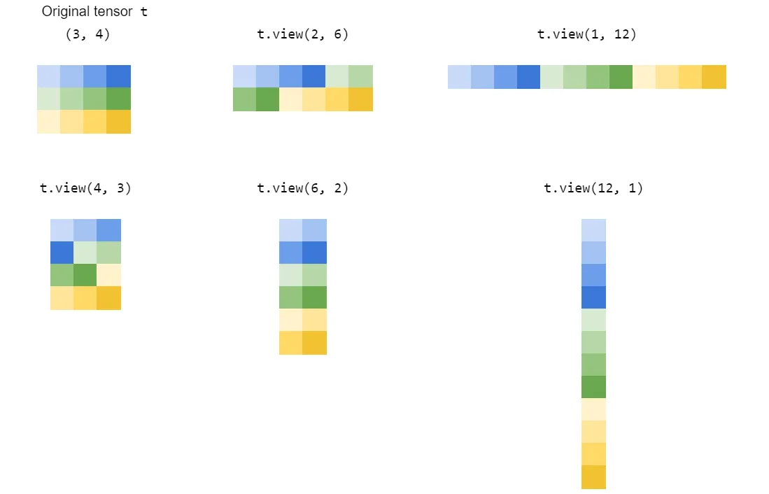
使用形状为(18,)的张量t，只能为以下形状创建新的视图：(1, 18)或等价地(1, -1)或(-1, 18)、(2, 9)或等价地(2, -1)或(-1, 9)、(3, 6)或等价地(3, -1)或(-1, 6)、(6, 3)或等价地(6, -1)或(-1, 3)、(9, 2)或等价地(9, -1)或(-1, 2)、(18, 1)或等价地(18, -1)或(-1, 1)。

从上面的形状元组中我们可以观察到，形状元组的元素相乘（例如2*9，3*6等）必须始终等于原张量中的元素总数（在我们的示例中为18）。

另一个需要注意的是，我们在每个形状元组中的一个位置使用了-1。通过使用-1，我们懒得自己进行计算，而是将任务委托给PyTorch在创建新的view时计算该值的计算。需要注意的一件重要事情是，我们只能在形状元组中使用单个-1。其余的值应由我们明确提供。否则，PyTorch会通过抛出RuntimeError来抱怨：

RuntimeError: only one dimension can be inferred

因此，对于上述所有形状，PyTorch将始终返回原张量t的新视图。这基本上意味着它只是更改了请求的每个新视图的张量的步幅信息。

下面是一些示例，说明如何随着每个新的view更改张量的步幅。

# stride of our original tensor `t`
In [53]: t.stride() 
Out[53]: (1,)

现在，我们将看到新的{{视图}}所需的步骤：

# shape (1, 18)
In [54]: t1 = t.view(1, -1)
# stride tensor `t1` with shape (1, 18)
In [55]: t1.stride() 
Out[55]: (18, 1)

# shape (2, 9)
In [56]: t2 = t.view(2, -1)
# stride of tensor `t2` with shape (2, 9)
In [57]: t2.stride()       
Out[57]: (9, 1)

# shape (3, 6)
In [59]: t3 = t.view(3, -1) 
# stride of tensor `t3` with shape (3, 6)
In [60]: t3.stride() 
Out[60]: (6, 1)

# shape (6, 3)
In [62]: t4 = t.view(6,-1)
# stride of tensor `t4` with shape (6, 3)
In [63]: t4.stride() 
Out[63]: (3, 1)

# shape (9, 2)
In [65]: t5 = t.view(9, -1) 
# stride of tensor `t5` with shape (9, 2)
In [66]: t5.stride()
Out[66]: (2, 1)

# shape (18, 1)
In [68]: t6 = t.view(18, -1)
# stride of tensor `t6` with shape (18, 1)
In [69]: t6.stride()
Out[69]: (1, 1)

那就是view()函数的神奇之处。对于每个新的视图，它只是改变了(原始)张量的步幅，只要新视图的形状与原始形状兼容即可。

从步幅元组中可以观察到另一个有趣的事情，即第0个位置上的元素值等于形状元组中第1个位置上的元素值。

In [74]: t3.shape 
Out[74]: torch.Size([3, 6])
                        |
In [75]: t3.stride()    |
Out[75]: (6, 1)         |
          |_____________|

这是因为：

In [76]: t3 
Out[76]: 
tensor([[ 0,  1,  2,  3,  4,  5],
        [ 6,  7,  8,  9, 10, 11],
        [12, 13, 14, 15, 16, 17]])

步幅(6, 1)表示在沿着第0个维度移动到下一个元素时，我们必须"跳"或者说走6步（例如，要从0到6，需要走6步）。但是在第1个维度中，我们只需要走一步（例如，要从2到3）。

因此，步幅信息是从内存中访问元素以执行计算的核心。

torch.reshape()

这个函数将返回一个视图，只要新形状与原始张量的形状兼容，就完全等同于使用torch.Tensor.view()。否则，它将返回一份副本。

然而，torch.reshape()的注意事项警告说：

连续输入和具有兼容步幅的输入可以在不复制的情况下重新整形，但不应依赖于复制与查看行为。

- kmario23

5

让我们通过以下示例来理解视图：

    a=torch.range(1,16)

print(a)

    tensor([ 1.,  2.,  3.,  4.,  5.,  6.,  7.,  8.,  9., 10., 11., 12., 13., 14.,
            15., 16.])

print(a.view(-1,2))

    tensor([[ 1.,  2.],
            [ 3.,  4.],
            [ 5.,  6.],
            [ 7.,  8.],
            [ 9., 10.],
            [11., 12.],
            [13., 14.],
            [15., 16.]])

print(a.view(2,-1,4))   #3d tensor

    tensor([[[ 1.,  2.,  3.,  4.],
             [ 5.,  6.,  7.,  8.]],

            [[ 9., 10., 11., 12.],
             [13., 14., 15., 16.]]])
print(a.view(2,-1,2))

    tensor([[[ 1.,  2.],
             [ 3.,  4.],
             [ 5.,  6.],
             [ 7.,  8.]],

            [[ 9., 10.],
             [11., 12.],
             [13., 14.],
             [15., 16.]]])

print(a.view(4,-1,2))

    tensor([[[ 1.,  2.],
             [ 3.,  4.]],

            [[ 5.,  6.],
             [ 7.,  8.]],

            [[ 9., 10.],
             [11., 12.]],

            [[13., 14.],
             [15., 16.]]])

-1作为参数值是计算某个变量（比如x）的一种简单方法，前提是我们已经知道了另一个变量（比如y或z）的值。对于三维情况，反过来也是一样的，在二维情况下，如果我们知道y的值，那么-1作为参数值就是计算x的一种简单方法，反之亦然。

- Lija Alex

很好的插图！ - WestCoastProjects

4

我发现x.view(-1, 16 * 5 * 5)等同于x.flatten(1)，其中参数1表示从第一维开始展平（不展平“样本”维度）。如您所见，后者的用法在语义上更清晰、更易于使用，因此我更喜欢flatten()。

- FENGSHI ZHENG

3

weights.reshape(a, b)将返回一个新的张量，其大小为（a，b），数据与weights相同，即它将数据复制到内存中的另一个位置。 weights.resize_(a, b)返回具有不同形状的相同张量。但是，如果新形状导致元素数量少于原始张量，则会从张量中删除一些元素（但不会从内存中删除）。如果新形状导致元素数量多于原始张量，则在内存中未初始化新元素。 weights.view(a, b)将返回一个新的张量，其大小为（a，b），数据与weights相同。

- Jibin Mathew

3

什么是参数-1的含义？

你可以将“-1”解读为动态数量的参数或“任何内容”。正因如此，在“view（）”中只能有一个参数“-1”。

如果你使用“x.view（-1,1）”，那么输出的张量形状将根据“x”的元素数量而定，为“[anything,1]”。例如：

import torch
x = torch.tensor([1, 2, 3, 4])
print(x,x.shape)
print("...")
print(x.view(-1,1), x.view(-1,1).shape)
print(x.view(1,-1), x.view(1,-1).shape)

会输出:

tensor([1, 2, 3, 4]) torch.Size([4])
...
tensor([[1],
        [2],
        [3],
        [4]]) torch.Size([4, 1])
tensor([[1, 2, 3, 4]]) torch.Size([1, 4])

- prosti

1

我非常喜欢@Jadiel de Armas的例子。

我想为.view(...)中元素排序添加一些见解：

对于形状为(a,b,c)的张量，它的元素顺序由编号系统确定：第一个数字有a个，第二个数字有b个，第三个数字有c个。
.view(...)返回的新张量中元素的映射保留了原始张量的顺序。

- ychnh

网页内容由stack overflow 提供, 点击上面的

可以查看英文原文，
原文链接

- Kashyap · Accepted Answer

view()重新整形张量，而不会复制内存，类似于numpy的reshape()。

给定一个有16个元素的张量a：

import torch
a = torch.range(1, 16)

要将此张量重塑为 4 x 4 张量，请使用：

a = a.view(4, 4)

现在a将是一个4 x 4的张量。请注意，重塑后元素的总数需要保持不变。将张量a重塑为3 x 5张量是不合适的。

-1参数的含义是什么？

如果您不知道要多少行，但确定列数，则可以使用-1指定列数。（请注意，您可以将其扩展到更多维的张量中。只能有一个轴值为-1）这是告诉库的一种方式：“给我一个具有这么多列的张量，并计算必要的行数以使此成为可能”。

在此模型定义代码中可以看到这一点。在前向函数中的x = self.pool（F.relu（self.conv2（x）））之后，您将拥有16深度特征映射。您必须将其展平以将其传递给完全连接的层。因此，您告诉PyTorch将您获得的张量重塑为具有特定列数的张量，并告诉它自己决定行数。

PyTorch中的.view()是什么意思？

-1参数的含义是什么？

view()如何工作？

PyTorch -1

torch.Tensor.view()

torch.reshape()

`view()`如何工作？

`torch.Tensor.view()`