使用相同的验证集对模型和CalibratedClassifierCV进行校准

Question

在CalibratedClassifierCV的文档中指出：“用于训练校准器的样本不应用于训练目标分类器。”据我理解，如果我们使用X_train来训练我们的模型，那么我们就不应该使用X_train来训练校准器（因为我认为它只是将X_train映射到model.predict_proba？）。但是，使用已用于超参数优化的验证集X_val来校准校准器是否公平呢？

- CutePoison

---

这个问题更适合在stats.SE或datascience.SE上提问。 - Ben Reiniger

Answer 1

CalibratedClassifierCV会在一部分数据上拟合分类器，然后查看预测概率是否与另一个数据集上的真实标签相对应。然后它尝试调整（“校准”）概率，使得对于具有0.7概率的一组样本，将有大约0.7个真实标签为“1”（用于二元分类）。

注意，训练分类器和拟合校准器是在不同的数据集上完成的，以考虑可能存在的偏差。这可以通过两种不同的方式完成：

1. CalibratedClassifierCV(..., cv=None, ensemble=True)。根据提供的cv策略划分您的训练数据，例如cv=5。像往常一样，您在k-1个折叠上训练基础估计器（要校准的分类器），然后在第k个剩下的折叠上拟合校准器。测试的结果预测将是k个已拟合校准器的平均值（“集成”）。

2. 如果ensemble=False，则使用单次拟合的cross_val_predict来拟合校准器。

有了这个理解：

使用已经用于超参数优化的验证集X_val来校准校准器是否公平？

您可以找到最佳的超参数，然后使用相同的训练数据集，但选择了CV策略(Ensemble True或False)来拟合校准器。请再次注意，您永远不会在同一数据上拟合分类器和校准器。

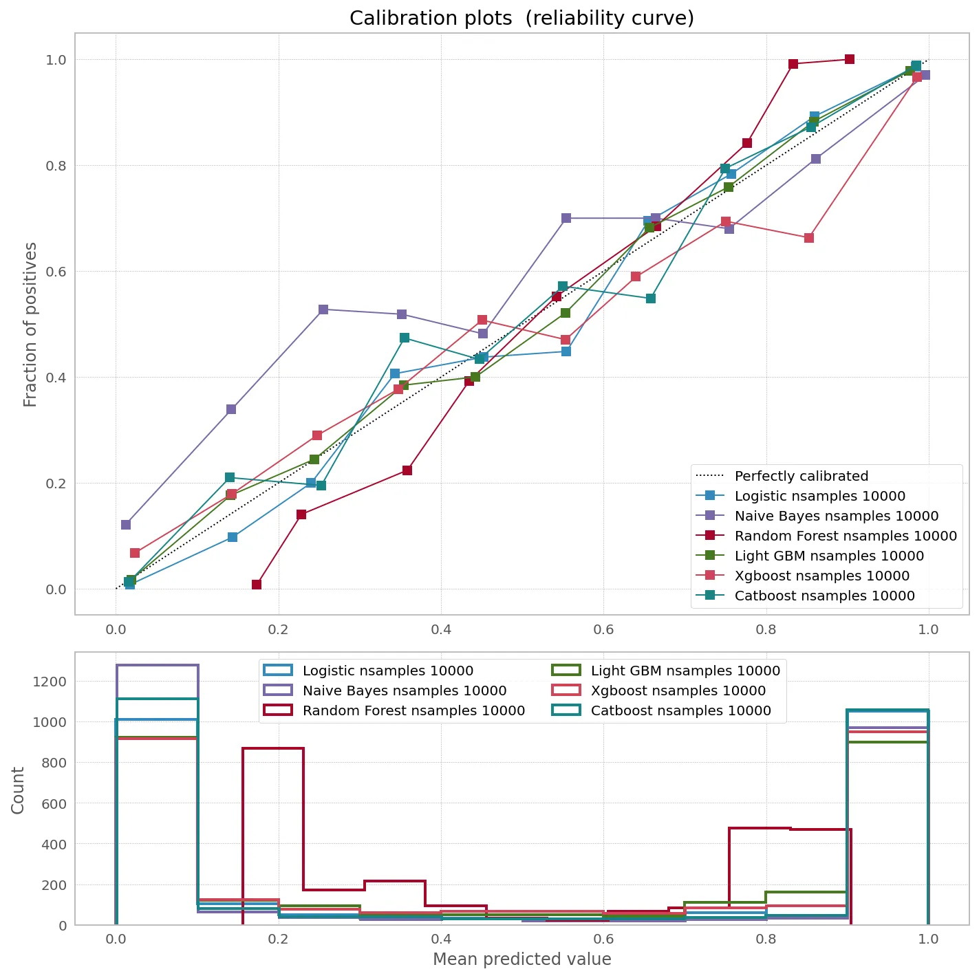
有趣的是，根据分类器和数据大小，校准可能会或可能不会帮助提高概率预测的准确性：

from sklearn import datasets
from sklearn.naive_bayes import GaussianNB
from sklearn.linear_model import LogisticRegression
from sklearn.ensemble import RandomForestClassifier
from sklearn.svm import SVC
from sklearn.calibration import calibration_curve, CalibratedClassifierCV
from xgboost import XGBClassifier
from lightgbm import LGBMClassifier
from catboost import CatBoostClassifier

np.random.seed(42)

# Create classifiers
lrc = LogisticRegression(n_jobs=-1)
gnb = GaussianNB()
svc = SVC(C=1.0, probability=True,)
rfc = RandomForestClassifier(n_estimators=300, max_depth=3,n_jobs=-1)
xgb = XGBClassifier(
    n_estimators=300,
    max_depth=3,
    objective="binary:logistic",
    eval_metric="logloss",
    use_label_encoder=False,
)
lgb = LGBMClassifier(n_estimators=300, objective="binary", max_depth=3)
cat = CatBoostClassifier(n_estimators=300, max_depth=3, objective="Logloss", verbose=0)

df = pd.DataFrame()

plt.figure(figsize=(10, 10))
ax1 = plt.subplot2grid((3, 1), (0, 0), rowspan=2)
ax2 = plt.subplot2grid((3, 1), (2, 0))
ax1.plot([0, 1], [0, 1], "k:", label="Perfectly calibrated")

for clf, name in [
    (lrc, "Logistic"),
    (gnb, "Naive Bayes"),
#     (svc, "Support Vector Classification"),
    (rfc, "Random Forest"),
    (lgb, "Light GBM"),
    (xgb, "Xgboost"),
    (cat, "Catboost"),
]:
    print(name)
    for nsamples in [1000,10000,100000]:
        train_samples = 0.75 
        X, y = make_classification(
            n_samples=nsamples, n_features=20, n_informative=2, n_redundant=2
        )
        i = int(train_samples * nsamples)
        X_train = X[:i]
        X_test  = X[i:]
        y_train = y[:i]
        y_test  = y[i:]
        clf.fit(X_train, y_train)
        prob_pos = clf.predict_proba(X_test)[:, 1]
        fraction_of_positives, mean_predicted_value = calibration_curve(
            y_test, prob_pos, n_bins=10
        )

        if nsamples in [10000]:
            ax1.plot(
                mean_predicted_value,
                fraction_of_positives,
                "s-",
                label="%s" % (name + " nsamples " + str(nsamples),),
            )

            ax2.hist(
                prob_pos,
                bins=10,
                label="%s" % (name + " nsamples " + str(nsamples),),
                histtype="step",
                lw=2,
            )

        preds = clf.predict_proba(X_test)
        ll_before = log_loss(y_test, preds)
        preds = (
            CalibratedClassifierCV(clf, cv=5)
            .fit(X_train, y_train)
            .predict_proba(X_test)
        )
        ll_after = log_loss(y_test, preds)
        df = df.append(pd.DataFrame({
            "Samples": [nsamples],
            "Model": name,
            "LogLoss Before": round(ll_before,4),
            "LogLoss After": round(ll_after,4),
            "Gain": round(ll_before/ll_after,4)
        }))

ax1.set_ylabel("Fraction of positives")
ax1.set_ylim([-0.05, 1.05])
ax1.legend(loc="lower right")
ax1.set_title("Calibration plots  (reliability curve)")

ax2.set_xlabel("Mean predicted value")
ax2.set_ylabel("Count")
ax2.legend(loc="upper center", ncol=2)

plt.tight_layout()
print(df)

---

   Samples          Model  LogLoss Before  LogLoss After    Gain
0     1000       Logistic          0.3941         0.3854  1.0226
0    10000       Logistic          0.1340         0.1345  0.9959
0   100000       Logistic          0.1645         0.1645  0.9999
0     1000    Naive Bayes          0.3025         0.2291  1.3206
0    10000    Naive Bayes          0.4094         0.3055  1.3403
0   100000    Naive Bayes          0.4119         0.2594  1.5881
0     1000  Random Forest          0.4438         0.3137  1.4146
0    10000  Random Forest          0.3450         0.2776  1.2427
0   100000  Random Forest          0.3104         0.1642  1.8902
0     1000      Light GBM          0.2993         0.2219  1.3490
0    10000      Light GBM          0.2074         0.2182  0.9507
0   100000      Light GBM          0.2397         0.2534  0.9459
0     1000        Xgboost          0.1870         0.1638  1.1414
0    10000        Xgboost          0.3072         0.2967  1.0351
0   100000        Xgboost          0.1136         0.1186  0.9575
0     1000       Catboost          0.1834         0.1901  0.9649
0    10000       Catboost          0.1251         0.1377  0.9085
0   100000       Catboost          0.1600         0.1727  0.9264

- Sergey Bushmanov