使用“与平均值的差异”模型来处理分类变量上的所有系数,需要使用“对比编码”吗?

10
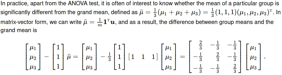
假设我们想做一个简单的“收入描述模型”。 假设我们有三个群体,北部、中部和南部(考虑美国地区)。 在比较其他相似的群体时,假设北部的平均收入为130,中部为80,南部为60。 假设群体大小相等,因此平均值为90。
在(线性回归)模型中,应该有一种方法来报告系数与总体平均数(在多元情况下,“所有其他条件相等”)之间的差异,并为每个系数得到一个: $ \beta_{North} = 40 $ $ \beta_{Central} = -10 $ $ \beta_{South} = -30 $
显然跳过截距。
这对我来说似乎最直观。但是,我无论如何都想不出如何使用R的“对比编码”来做到这一点。(而且,这似乎会搞乱变量名)。
设置我的模拟/ mwe的参数
m_inc <- 90
b_n <- 40
b_c  <- -10
b_s <- -30

sd_prop <- 0.5 #sd as share of mean
pop_per <- 1000 

模拟数据

set.seed(100)

n_income <- rnorm(pop_per, m_inc + b_n, (m_inc + b_n)*sd_prop)
c_income <- rnorm(pop_per, m_inc + b_c, (m_inc + b_s)*sd_prop)
s_income <- rnorm(pop_per, m_inc + b_s, (m_inc + b_s)*sd_prop)

noise_var <- rnorm(pop_per*3, 0, (m_inc + b_s)*sd_prop)

i_df <- tibble(
  region = rep( c("n", "c", "s"), c(pop_per, pop_per, pop_per) ),
  income = c(n_income, c_income, s_income),
  noise_var
) %>% 
  mutate(region = as.factor(region))


i_df %>%                               # Summary by group using purrr
  split(.$region) %>%
  purrr::map(summary)

看起来已经足够接近了。

现在我想要“建立收入模型”以便控制其他因素并通过地区比较差异。为了说明这个问题,让我们将南部设为基准组。我设置了默认的contr.treatment,以防您对其进行了重置。


i_df <- i_df %>%   mutate(region = relevel(region, ref="s"))
options(contrasts = rep ("contr.treatment", 2))


(
  basic_lm <- i_df %>% lm(income ~ region + noise_var, .)
)

标准做法:拦截器(intercept)是(大致上)“基础组”南方的均值,而系数regioncregionn则分别表示这些地区的相对调整,大约为+20和+70。

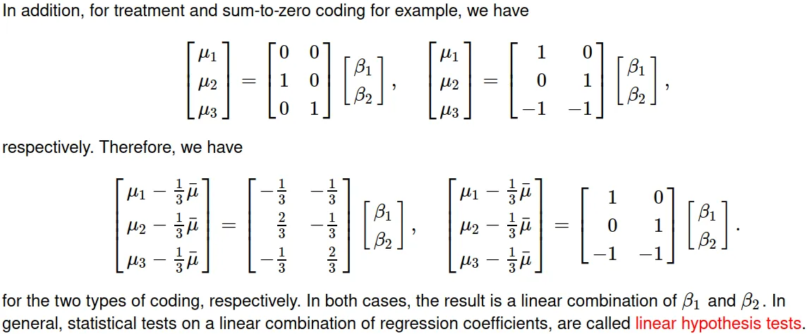
这是标准的“虚拟编码”或“处理编码”,在R中是默认设置。

我们可以将此默认设置(针对无序变量)调整为称为“总和对比编码”的东西,适用于无序和有序变量。

options(contrasts = rep ("contr.sum", 2))

(
  basic_lm_cc <- i_df %>% lm(income ~ region + noise_var, .)
)

现在看起来我们得到了所需的调整系数,但是:

  1. 地区名称丢失了;我怎么知道哪个是哪个?
  2. 显然报告的是 s(南部)和 c(中部)的调整系数。不太直观。

无论如何重新设置地区以设置特定基本组(我尝试过)... 系数都不会改变。

我找到了一个解决方案,但这不是“正确的方法”。我让结果(收入)变量减去平均值,并强制截距为0:


i_df %>% 
  mutate(m_inc = mean(income)) %>% 
 lm(income - m_inc ~ 0  + region + noise_var, .)

太好了!这正是我想要的,而且变量名也奇迹般地保留下来了。但这似乎是一种奇怪的方法。还要注意,使用上面的代码,无论是求和对比矩阵还是处理对比矩阵,都将出现这组系数。

如何使用对比编码或其他工具以“正确”的方式完成此操作?


这是一个好问题,如果我有机会/没有其他人介入,明天我会帮忙的。 - Ben Bolker
谢谢。请注意,我稍微编辑了示例,使其不对称。 - daaronr
当您有多个类别时,这也不容易工作。 - daaronr
唉,我还没有答案。emmeans::emmeans(basic_lm, ~region, offset=-mean(i_df$income)) 给出了正确的值,但是标准误差却不对。 - Ben Bolker
1个回答

9
无法使用对比编码来实现这个目的。在一元方差分析中,对比用于将一个 N-水平因子编码为 N - 1 个变量加上一个截距,因此仍然有 N 个变量到 N 个变量。但是,在模型中同时包括组均值的总体均值和偏差是从 N 个变量到 N + 1 个变量的重新参数化。即使我们找到了方法,这会使设计矩阵秩缺失,并且lm/aov/glm等函数将一个变量放置为 NA
一般情况下,我们必须进行后续统计分析。在本答案中,我将总结对比编码的作用,并展示四种比较组均值和总体均值的方法:手动编码、使用multcompemmeanscar
library(ggplot2)
library(car)
library(multcomp)
library(emmeans)

设置

我将使用与您类似的例子。

setup

SimData <- function (group.size, group.mean, group.variance) {
  ## number of groups
  ng <- length(group.size)
  if (ng > 5) stop("There is no need to experiment that many groups!")
  ## number of observations per group
  n <- sum(group.size)
  ## generate a factor variable 'f' for these groups
  f <- rep.int(factor(sprintf("G%d", 1:ng)), group.size)
  ## simulate samples from each group
  mu <- rep.int(group.mean, group.size)
  se <- rep.int(sqrt(group.variance), group.size)
  y <- rnorm(n, mu, se)
  ## numerical covariate 'x' with slope = 1
  lim <- sd(y)
  br <- seq.int(-lim, lim, length.out = ng + 1)
  interval <- cbind(br[-(ng + 1)], br[-1])
  interval <- interval[sample.int(ng), ]
  a <- rep.int(interval[, 1], group.size)
  b <- rep.int(interval[, 2], group.size)
  x <- runif(n, a, b)
  ## create data.frame
  data.frame(y = y + x, f = f, x = x)
}

set.seed(4891738)  ## my Stack Overflow ID
group.size <- c(100, 125, 150)
group.mean <- c(130, 80, 60)
group.variance <- 0.25 * group.mean
dat <- SimData(group.size, group.mean, group.variance)

ggplot(data = dat, mapping = aes(x = x, y = y, colour = f)) + geom_point()

data

对于每个组进行朴素的平均值和方差计算是误导性的,因为我们离真相相距甚远!

## true values are 130, 80, 60
with(dat, tapply(y, f, mean))
##        G1        G2        G3 
## 148.36985  60.38273  59.45486

## true values are 32.5, 20 and 15
with(dat, tapply(y, f, var))
##       G1       G2       G3 
## 67.37108 55.25185 41.69867

对比编码

形式直观表达

实际表达

## treatment coding
contr.treatment(3)
##   2 3
## 1 0 0
## 2 1 0
## 3 0 1

## sum-to-zero coding
contr.sum(3)
##   [,1] [,2]
## 1    1    0
## 2    0    1
## 3   -1   -1

why summary table does not display all levels

fit.treatment <- lm(y ~ f + x, dat, contrasts = list(f = "contr.treatment"))
coef(fit.treatment)
#(Intercept)         fG2         fG3           x 
#  128.94609   -48.71525   -69.03433     1.03121 

summary(fit.treatment)
anova(fit.treatment)

fit.sum <- lm(y ~ f + x, dat, contrasts = list(f = "contr.sum"))
coef(fit.sum)
#(Intercept)          f1          f2           x 
#  89.696234   39.249860   -9.465391    1.031210 

summary(fit.sum)
anova(fit.sum)

请注意,尽管使用不同的对比度编码会产生不同的回归系数,但由于生成相同的拟合值,它们实际上是等价的。
all.equal(fit.treatment$fitted.values, fit.sum$fitted.values)
## [1] TRUE

使用总体均值比较群体均值

线性假设检验1

线性假设检验2

R中的线性假设检验

1. 不使用 fancy package 的基础方法

基础方法

## 3 x 2 linear combination matrix
wt.treatment <- matrix(c(-1, 2, -1, -1, -1, 2), nrow = 3) / 3
wt.sum <- matrix(c(1, 0, -1, 0, 1, -1), nrow = 3)

vanilla <- function (wt, beta.ind, lmfit) {
  ## beta coefficients and their covariance matrix
  beta <- coef(lmfit)[beta.ind]
  V <- vcov(lmfit)[beta.ind, beta.ind]
  ## linear combination and their standard errors
  MEAN <- c(wt %*% beta)
  ## get standard errors for sum of `LinearComb`
  SE <- sqrt(diag(wt %*% tcrossprod(V, wt)))
  ## perform t-test
  tscore <- MEAN / SE
  pvalue <- 2 * pt(abs(tscore), lmfit$df.residual, lower.tail = FALSE)
  ## return a matrix
  ans <- matrix(c(MEAN, SE, tscore, pvalue), ncol = 4L)
  colnames(ans) <- c("Estimate", "Std. Error", "t value", "Pr(>|t|)")
  printCoefmat(ans)
}

vanilla(wt.treatment, 2:3, fit.treatment)
##       Estimate Std. Error t value  Pr(>|t|)    
## [1,]  39.24986    0.90825  43.215 < 2.2e-16 ***
## [2,]  -9.46539    0.89404 -10.587 < 2.2e-16 ***
## [3,] -29.78447    0.32466 -91.741 < 2.2e-16 ***
## ---
## Signif. codes:  0 '***' 0.001 '**' 0.01 '*' 0.05 '.' 0.1 ' ' 1

vanilla(wt.sum, 2:3, fit.sum)  ## identical to above

2. 使用'multcomp'软件包

multcomp

## pad columns of zeros to zero out the effect of alpha and gamma
wt.treatment0 <- cbind(0, wt.treatment, 0)
wt.sum0 <- cbind(0, wt.sum, 0)

summary(glht(fit.treatment, linfct = wt.treatment0))
## Linear Hypotheses:
##        Estimate Std. Error t value Pr(>|t|)    
## 1 == 0  39.2499     0.9083   43.22   <2e-16 ***
## 2 == 0  -9.4654     0.8940  -10.59   <2e-16 ***
## 3 == 0 -29.7845     0.3247  -91.74   <2e-16 ***
## ---
## Signif. codes:  0 '***' 0.001 '**' 0.01 '*' 0.05 '.' 0.1 ' ' 1
## (Adjusted p values reported -- single-step method)

summary(glht(fit.sum, linfct = wt.sum0))  ## identical to above

3. 使用‘emmeans’包

emmeans

emmeans(fit.treatment, specs = eff ~ f)
## $emmeans
##  f  emmean    SE  df lower.CL upper.CL
##  G1  127.3 1.002 371    125.4    129.3
##  G2   78.6 0.874 371     76.9     80.3
##  G3   58.3 0.379 371     57.5     59.0
## 
## Confidence level used: 0.95 
## 
## $contrasts
##  contrast  estimate    SE  df t.ratio p.value
##  G1 effect    39.25 0.908 371  43.215  <.0001
##  G2 effect    -9.47 0.894 371 -10.587  <.0001
##  G3 effect   -29.78 0.325 371 -91.741  <.0001
## 
## P value adjustment: fdr method for 3 tests

emmeans(fit.sum, specs = eff ~ f)  ## identical to above

specs = ~fspecs = "f"时,只有$emmeans(边际均值)组件被报告。左侧的"eff"意味着需要调用eff.emmc()来应用对比,$contrasts组件呈现了这样的结果。

4. 使用‘car’包

cars中的linearHypothesis()函数执行F检验,以测试所有线性组合是否同时为0。因此,它与上述演示中的t检验不同。此外,它会给出误差:

linearHypothesis(fit.treatment, hypothesis.matrix = wt.treatment0)
#Error in solve.default(vcov.hyp) : 
#  system is computationally singular: reciprocal condition number = 1.12154e-17

linearHypothesis(fit.sum, hypothesis.matrix = wt.sum0)  ## identical to above

这个回答在某种意义上是我之前几个答案的总结.


网页内容由stack overflow 提供, 点击上面的
可以查看英文原文,
原文链接