我已经写了一个例程,将点数据插值到正规的网格上。然而,我发现
相关代码包括如何构建插值器。
我正在运行的示例有27个输入插值值点,我要在接近20000 X 20000的网格上进行插值(我是按内存块大小来处理的,所以不会让电脑爆炸)。下面是我在相关代码上运行的两个cProfile结果。请注意,最近邻方案需要406秒,而线性方案需要256秒。最近邻方案受到scipy的kdTree调用的影响,这似乎是合理的,但rbf的表现却比它快得多。你有什么想法或者我能做些什么来使我的最近邻方案比线性方案更快?下面是线性情况的运行结果:
scipy 的最近邻插值实现速度几乎比我用于线性插值的径向基函数 (scipy.interpolate.Rbf) 慢两倍。相关代码包括如何构建插值器。
if interpolation_mode == 'linear':
    interpolator = scipy.interpolate.Rbf(
        point_array[:, 0], point_array[:, 1], value_array,
        function='linear', smooth=.01)
elif interpolation_mode == 'nearest':
    interpolator = scipy.interpolate.NearestNDInterpolator(
        point_array, value_array)
当调用插值时
result = interpolator(col_coords.ravel(), row_coords.ravel())
我正在运行的示例有27个输入插值值点,我要在接近20000 X 20000的网格上进行插值(我是按内存块大小来处理的,所以不会让电脑爆炸)。下面是我在相关代码上运行的两个cProfile结果。请注意,最近邻方案需要406秒,而线性方案需要256秒。最近邻方案受到scipy的kdTree调用的影响,这似乎是合理的,但rbf的表现却比它快得多。你有什么想法或者我能做些什么来使我的最近邻方案比线性方案更快?下面是线性情况的运行结果:
     25362 function calls in 225.886 seconds

   Ordered by: internal time
   List reduced from 328 to 10 due to restriction <10>

   ncalls  tottime  percall  cumtime  percall filename:lineno(function)
      253  169.302    0.669  207.516    0.820 C:\Python27\lib\site-packages\scipy\interpolate\rbf.py:112(
_euclidean_norm)
      258   38.211    0.148   38.211    0.148 {method 'reduce' of 'numpy.ufunc' objects}
      252    6.069    0.024    6.069    0.024 {numpy.core._dotblas.dot}
        1    5.077    5.077  225.332  225.332 C:\Python27\lib\site-packages\pygeoprocessing-0.3.0a8.post2
8+n5b1ee2de0d07-py2.7-win32.egg\pygeoprocessing\geoprocessing.py:333(interpolate_points_uri)
      252    1.849    0.007    2.137    0.008 C:\Python27\lib\site-packages\numpy\lib\function_base.py:32
85(meshgrid)
      507    1.419    0.003    1.419    0.003 {method 'flatten' of 'numpy.ndarray' objects}
     1268    1.368    0.001    1.368    0.001 {numpy.core.multiarray.array}
      252    1.018    0.004    1.018    0.004 {_gdal_array.BandRasterIONumPy}
        1    0.533    0.533  225.886  225.886 pygeoprocessing\tests\helper_driver.py:10(interpolate)
      252    0.336    0.001  216.716    0.860 C:\Python27\lib\site-packages\scipy\interpolate\rbf.py:225(
__call__)
最近邻运行:
     27539 function calls in 405.624 seconds

   Ordered by: internal time
   List reduced from 309 to 10 due to restriction <10>

   ncalls  tottime  percall  cumtime  percall filename:lineno(function)
      252  397.806    1.579  397.822    1.579 {method 'query' of 'ckdtree.cKDTree' objects}
      252    1.875    0.007    1.881    0.007 {scipy.interpolate.interpnd._ndim_coords_from_arrays}
      252    1.831    0.007    2.101    0.008 C:\Python27\lib\site-packages\numpy\lib\function_base.py:3285(meshgrid)
      252    1.034    0.004  400.739    1.590 C:\Python27\lib\site-packages\scipy\interpolate\ndgriddata.py:60(__call__)
        1    1.009    1.009  405.030  405.030 C:\Python27\lib\site-packages\pygeoprocessing-0.3.0a8.post28+n5b1ee2de0d07-py2.7-win32.egg\pygeoprocessing\geoprocessing.py:333(interpolate_points_uri)
      252    0.719    0.003    0.719    0.003 {_gdal_array.BandRasterIONumPy}
        1    0.509    0.509  405.624  405.624 pygeoprocessing\tests\helper_driver.py:10(interpolate)
      252    0.261    0.001    0.261    0.001 {numpy.core.multiarray.copyto}
       27    0.125    0.005    0.125    0.005 {_ogr.Layer_CreateFeature}
        1    0.116    0.116    0.254    0.254 C:\Python27\lib\site-packages\pygeoprocessing-0.3.0a8.post28+n5b1ee2de0d07-py2.7-win32.egg\pygeoprocessing\geoprocessing.py:362(_parse_point_data)
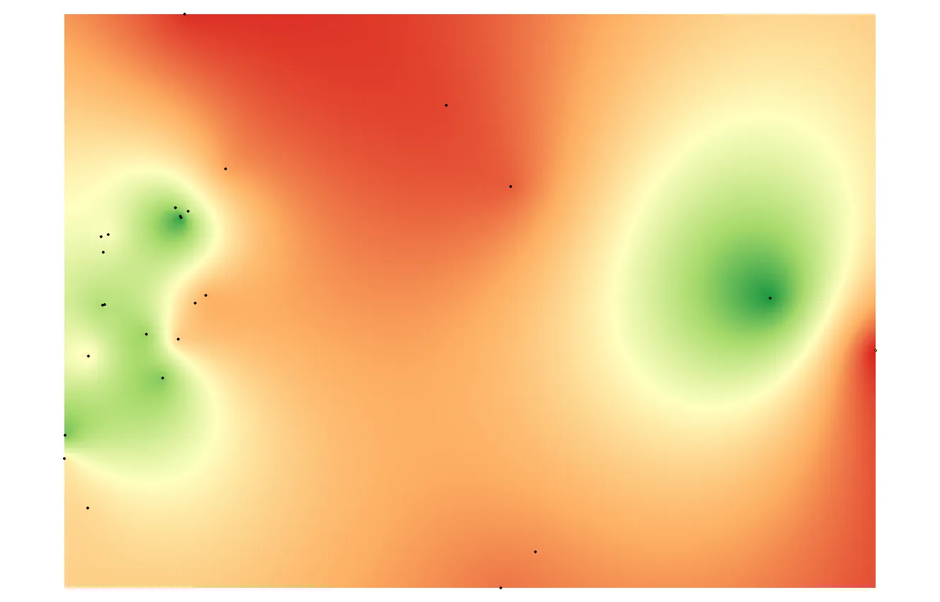
供参考,我还包括这两个测试用例的可视化结果。
最近邻

线性