ggplot置信区间未填充整个线性混合模型数据集

Question

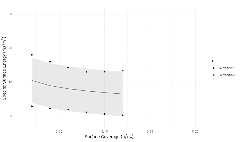
我的 ggplot R 代码在其他数据集上完美运行，但我对于为什么它在一个特定的数据集上无法正常工作感到困惑。请参见下面的图像，其中填充置信区间停止于 0.10：

复现问题：

library(nlme)
library(ggeffects)
library(ggplot2)
SurfaceCoverage <- c(0.02,0.04,0.06,0.08,0.1,0.12,0.02,0.04,0.06,0.08,0.1,0.12)
SpecificSurfaceEnergy <- c(18.0052997,15.9636971,14.2951057,13.0263081,13.0816591,13.3825573,2.9267577,2.2889628,1.8909175,1.0083036,0.5683574,0.1681063)
sample <- c(1,1,1,1,1,1,2,2,2,2,2,2)

highW <- data.frame(sample,SurfaceCoverage,SpecificSurfaceEnergy)

highW$sample <- sub("^", "Wettable", highW$sample)
highW$RelativeHumidity <- "High relative humidity"; highW$group <- "Wettable"
highW$sR <- paste(highW$sample,highW$RelativeHumidity)

dfhighW <- data.frame(
  "y"=c(highW$SpecificSurfaceEnergy),
  "x"=c(highW$SurfaceCoverage),
  "b"=c(highW$sample),
  "sR"=c(highW$sR)
)

mixed.lme <- lme(y~log(x),random=~1|b,data=dfhighW)
pred.mmhighW <- ggpredict(mixed.lme, terms = c("x"))

(ggplot(pred.mmhighW) + 
    geom_line(aes(x = x, y = predicted)) +          # slope
    geom_ribbon(aes(x = x, ymin = predicted - std.error, ymax = predicted + std.error), 
                fill = "lightgrey", alpha = 0.5) +  # error band
    geom_point(data = dfhighW,                      # adding the raw data (scaled values)
               aes(x = x, y = y, shape = b)) + 
    xlim(0.01,0.2) + 
    ylim(0,30) +
    labs(title = "") + 
    ylab(bquote('Specific Surface Energy ' (mJ/m^2))) +
    xlab(bquote('Surface Coverage ' (n/n[m]) )) +
    theme_minimal()
)

有人能给我建议如何解决这个问题吗？谢谢。

- Catalyst

Answer 1

由于您已将其从图表中排除，因此您的带状图的最后一部分已经消失。 您的带状图的下边缘是以下向量：

pred.mmhighW$predicted - pred.mmhighW$std.error
#> [1]  3.91264018  2.37386628  1.47061258  0.82834206  0.32935718 -0.07886245

请注意最终值为一个小负数，但您已设置y轴限制为：

ylim(0, 30)

所以任何负面的东西都将被切断。如果你改变为

ylim(-2, 30)

你将会获得：

- Allan Cameron

---

谢谢@Allan Cameron！！！！天啊，我总是犯这么简单的错误。你救了我的一天。另外，我可能需要休息一下，以便有一个清醒的眼睛来解决这个问题。再次感谢！ - Catalyst

Answer 2

我不知道是否已经回答过这个问题，但是coord_cartesian和scales::squish都是解决这个问题的两种方法。

• coord_cartesian调整视口而不会调整网格线等间距（不像xlim()/scale_*_continuous(limits = ...)，它们会“缩放”）
• scales::squish()如果你只是“压缩”无边框多边形而不是线条和点，那么效果不佳（对于填充/多边形的情况，压缩和裁剪产生相同的结果）。

gg0 <- (ggplot(pred.mmhighW) 
    + geom_ribbon(aes(x = x, ymin = predicted - std.error,
                      ymax = predicted + std.error), 
                  fill = "lightgrey", alpha = 0.5)
    + theme_minimal()
)

## set lower limit to 5 for a more obvious effect
gg0 + coord_cartesian(ylim = c(5, 30))
gg0 + scale_y_continuous(limits = c(5, 30),
                         ## oob = "out of bounds" behaviour
                         oob = scales::squish)

- Ben Bolker

---

这几乎与 https://stackoverflow.com/questions/57000066/clip-only-1-axis-using-coord-cartesian/57002219#57002219 相同。 - Ben Bolker