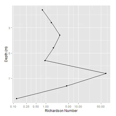
更新的解决方案
从 ggplot 2.2.0 开始,可以在面板顶部(和/或面板右侧)绘制坐标轴。
library(ggplot2)

depth = c(1.6,2.6,3.6, 4.6,5.6,6.6,7.6,8.6)
ri <- c(0.790143779,1.485888068,2.682375391,1.728120227,0.948414515,71.43308158,4.416120653,0.125458801)
df = data.frame(depth,ri)

m <- qplot(ri, depth, data=df) +
   scale_x_log10("Richardson Number",breaks = c(0.1,0.25,0.5,1,5,10, 50),
         position = "top") +
   scale_y_reverse("Depth (m)")+
   geom_path()
原始解决方案 经过对ggplot版本2.2.0的一些更新后。
可以使用gtable函数移动轴。从@Walter的答案这里调整代码,基本思路是:获取轴(轴标签和刻度线);反转轴标签和刻度线;在绘图面板上方立即添加一个新行到gtable布局中;将修改后的轴插入新行。
library(ggplot2)
library(gtable)
library(grid)
depth = c(1.6,2.6,3.6, 4.6,5.6,6.6,7.6,8.6)
ri <- c(0.790143779,1.485888068,2.682375391,1.728120227,0.948414515,71.43308158,4.416120653,0.125458801)
df = data.frame(depth,ri)
m <- qplot(ri, depth, data=df) +
scale_x_log10("Richardson Number",breaks = c(0.1,0.25,0.5,1,5,10, 50)) +
scale_y_reverse("Depth (m)")+
geom_path()
g1 <- ggplotGrob(m)
pp <- c(subset(g1$layout, name == "panel", se = t:r))
vinvert_title_grob <- function(grob) {
heights <- grob$heights
grob$heights[1] <- heights[3]
grob$heights[3] <- heights[1]
grob$vp[[1]]$layout$heights[1] <- heights[3]
grob$vp[[1]]$layout$heights[3] <- heights[1]
grob$children[[1]]$hjust <- 1 - grob$children[[1]]$hjust
grob$children[[1]]$vjust <- 1 - grob$children[[1]]$vjust
grob$children[[1]]$y <- unit(1, "npc") - grob$children[[1]]$y
grob
}
index <- which(g1$layout$name == "xlab-b")
xlab <- g1$grobs[[index]]
xlab <- vinvert_title_grob(xlab)
g1 <- gtable_add_rows(g1, g1$heights[g1$layout[index, ]$t], pp$t-1)
g1 <- gtable_add_grob(g1, xlab, pp$t, pp$l, pp$t, pp$r, clip = "off", name="topxlab")
index <- which(g1$layout$name == "axis-b")
xaxis <- g1$grobs[[index]]
ticks <- xaxis$children[[2]]
ticks$heights <- rev(ticks$heights)
ticks$grobs <- rev(ticks$grobs)
plot_theme <- function(p) {
plyr::defaults(p$theme, theme_get())
}
tml <- plot_theme(m)$axis.ticks.length
ticks$grobs[[2]]$y <- ticks$grobs[[2]]$y - unit(1, "npc") + tml
ticks$grobs[[1]] <- vinvert_title_grob(ticks$grobs[[1]])
xaxis$children[[2]] <- ticks
g1 <- gtable_add_rows(g1, g1$heights[g1$layout[index, ]$t], pp$t)
g1 <- gtable_add_grob(g1, xaxis, pp$t+1, pp$l, pp$t+1, pp$r, clip = "off", name = "axis-t")
g1 = g1[-c(9,10), ]
grid.newpage()
grid.draw(g1)
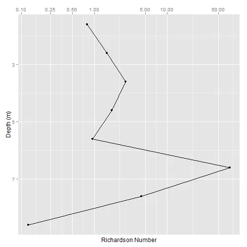

geom_path函数会按照您的要求用线连接点。调换轴的位置是ggplot2难以处理的问题,尽管可能可以实现,但并不简单,参见 https://dev59.com/dF8d5IYBdhLWcg3waxvo。 - tkmckenzie