回答如何在两层多层感知器中更新学习率?的问题:
考虑XOR问题:
X = xor_input = np.array([[0,0], [0,1], [1,0], [1,1]])
Y = xor_output = np.array([[0,1,1,0]]).T
一个简单的
- 两层多层感知器(MLP),它们之间使用sigmoid激活函数,
- 均方误差(MSE)作为损失函数/优化标准
如果我们从头开始训练模型:
from itertools import chain
import matplotlib.pyplot as plt
import numpy as np
np.random.seed(0)

def sigmoid(x): # Returns values that sums to one.
    return 1 / (1 + np.exp(-x))

def sigmoid_derivative(sx):
    # See https://math.stackexchange.com/a/1225116
    return sx * (1 - sx)

# Cost functions.
def mse(predicted, truth):
    return 0.5 * np.mean(np.square(predicted - truth))

def mse_derivative(predicted, truth):
    return predicted - truth

X = xor_input = np.array([[0,0], [0,1], [1,0], [1,1]])
Y = xor_output = np.array([[0,1,1,0]]).T

# Define the shape of the weight vector.
num_data, input_dim = X.shape
# Lets set the dimensions for the intermediate layer.
hidden_dim = 5
# Initialize weights between the input layers and the hidden layer.
W1 = np.random.random((input_dim, hidden_dim))

# Define the shape of the output vector.
output_dim = len(Y.T)
# Initialize weights between the hidden layers and the output layer.
W2 = np.random.random((hidden_dim, output_dim))

# Initialize weigh
num_epochs = 5000
learning_rate = 0.3

losses = []

for epoch_n in range(num_epochs):
    layer0 = X
    # Forward propagation.

    # Inside the perceptron, Step 2.
    layer1 = sigmoid(np.dot(layer0, W1))
    layer2 = sigmoid(np.dot(layer1, W2))

    # Back propagation (Y -> layer2)

    # How much did we miss in the predictions?
    cost_error = mse(layer2, Y)
    cost_delta = mse_derivative(layer2, Y)

    #print(layer2_error)
    # In what direction is the target value?
    # Were we really close? If so, don't change too much.
    layer2_error = np.dot(cost_delta, cost_error)
    layer2_delta = cost_delta *  sigmoid_derivative(layer2)

    # Back propagation (layer2 -> layer1)
    # How much did each layer1 value contribute to the layer2 error (according to the weights)?
    layer1_error = np.dot(layer2_delta, W2.T)
    layer1_delta = layer1_error * sigmoid_derivative(layer1)

    # update weights
    W2 += - learning_rate * np.dot(layer1.T, layer2_delta)
    W1 += - learning_rate * np.dot(layer0.T, layer1_delta)
    #print(np.dot(layer0.T, layer1_delta))
    #print(epoch_n, list((layer2)))

    # Log the loss value as we proceed through the epochs.
    losses.append(layer2_error.mean())
    #print(cost_delta)


# Visualize the losses
plt.plot(losses)
plt.show()
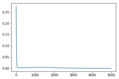
我们在第0轮迭代中损失急剧下降,然后迅速饱和:
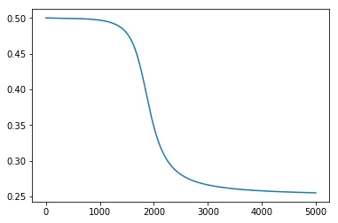
但是,如果我们使用pytorch训练类似的模型,训练曲线在饱和之前会逐渐下降:
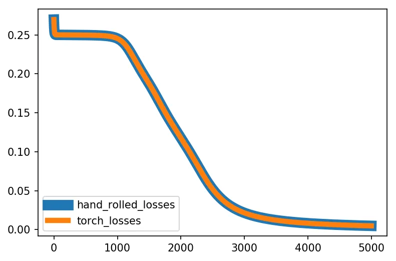
从零开始的MLP和PyTorch代码有什么区别?
为什么它在不同的收敛点实现收敛?
除了权重初始化之外,在从头开始的代码中使用的np.random.rand()和默认的torch初始化,我似乎看不到模型上的区别。
PyTorch代码:
from tqdm import tqdm
import numpy as np

import torch
from torch import nn
from torch import tensor
from torch import optim

import matplotlib.pyplot as plt

torch.manual_seed(0)
device = 'gpu' if torch.cuda.is_available() else 'cpu'

# XOR gate inputs and outputs.
X = xor_input = tensor([[0,0], [0,1], [1,0], [1,1]]).float().to(device)
Y = xor_output = tensor([[0],[1],[1],[0]]).float().to(device)


# Use tensor.shape to get the shape of the matrix/tensor.
num_data, input_dim = X.shape
print('Inputs Dim:', input_dim) # i.e. n=2

num_data, output_dim = Y.shape
print('Output Dim:', output_dim)
print('No. of Data:', num_data) # i.e. n=4

# Step 1: Initialization.

# Initialize the model.
# Set the hidden dimension size.
hidden_dim = 5
# Use Sequential to define a simple feed-forward network.
model = nn.Sequential(
            # Use nn.Linear to get our simple perceptron.
            nn.Linear(input_dim, hidden_dim),
            # Use nn.Sigmoid to get our sigmoid non-linearity.
            nn.Sigmoid(),
            # Second layer neurons.
            nn.Linear(hidden_dim, output_dim),
            nn.Sigmoid()
        )
model

# Initialize the optimizer
learning_rate = 0.3
optimizer = optim.SGD(model.parameters(), lr=learning_rate)

# Initialize the loss function.
criterion = nn.MSELoss()

# Initialize the stopping criteria
# For simplicity, just stop training after certain no. of epochs.
num_epochs = 5000

losses = [] # Keeps track of the loses.

# Step 2-4 of training routine.

for _e in tqdm(range(num_epochs)):
    # Reset the gradient after every epoch.
    optimizer.zero_grad()
    # Step 2: Foward Propagation
    predictions = model(X)

    # Step 3: Back Propagation
    # Calculate the cost between the predictions and the truth.
    loss = criterion(predictions, Y)
    # Remember to back propagate the loss you've computed above.
    loss.backward()

    # Step 4: Optimizer take a step and update the weights.
    optimizer.step()

    # Log the loss value as we proceed through the epochs.
    losses.append(loss.data.item())


plt.plot(losses)
---> 60 layer1_error = np.dot(layer2_delta, W2.T) ..... ValueError: shapes (4,50) and (1,5) not aligned: 50 (dim 1) != 1 (dim 0)。 - cs950.0,对吧?这是否意味着PyTorch代码有问题? @coldspeed 我能够从零开始的代码中复现OP的结果。当你运行它时,似乎layer2_delta以(4,50)的形状结束(对我来说,layer2_delta.shape是(4,1))。 - tel