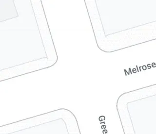
我正在使用OSM数据创建矢量街道地图。对于道路,我使用OSM提供的线几何体,并添加缓冲区将线转换为类似道路的几何体。
我的问题与几何体有关,而不是OSM,因此我将使用基本线来简化。
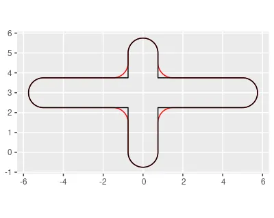
这将产生类似于以下内容:
是否有简单/实用的解决方案,或者我最好习惯于未圆形交叉?
谢谢
更新:
Lovalery和mrhellmann提出了两个解决方案。
最终,我选择了mrhellmann的答案,因为它符合我的特定需求;然而,我比较和探索了每个方法的优点,我分享如下。我将这个讨论留在这里,因为其他人可能有稍微不同的用例,了解差异是有用的。
让我们定义所使用的不同方法:
Lovalery 提出了一个好问题,负缓冲方法也可以使端点/极端值更平滑。
比较这三种方法表明,负缓冲方法影响的不仅是端盖,它会将几何体从所有侧面收缩 st_buffer 中使用的距离。
最后,要挑剔一下,
正如Lovalery所提到的,这取决于个体使用情况最好的选择。此外,普通观众是否会注意到街道比OSM说的短一米,或者曲线略微不对称?精度就像图形一样有趣...完美的精度可能并不重要,但它涉及到数学和数字,所以感觉应该很重要。
以上所有代码:
我的问题与几何体有关,而不是OSM,因此我将使用基本线来简化。
library(dplyr)
library(ggplot2)
library(sf)

# two lines representing an intersection of roads
l1 <- st_as_sfc(c("LINESTRING(0 0,0 5)","LINESTRING(-5 3,5 3)"))

# union the two lines (so they "intersect" instead of overlap once buffered
l2 <- l1 %>% st_union()

ggplot()+
  geom_sf(data = st_buffer(l2, dist = 0.75))
这将产生类似于以下内容:
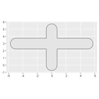
是否有简单/实用的解决方案,或者我最好习惯于未圆形交叉?
谢谢
更新:
Lovalery和mrhellmann提出了两个解决方案。
最终,我选择了mrhellmann的答案,因为它符合我的特定需求;然而,我比较和探索了每个方法的优点,我分享如下。我将这个讨论留在这里,因为其他人可能有稍微不同的用例,了解差异是有用的。
让我们定义所使用的不同方法:
l1 <- st_as_sfc(c("LINESTRING(0 0,0 5)","LINESTRING(-5 3,5 3)"))
l2 <- l1 %>% st_union()

l2.base <- l2 %>% st_buffer(dist = 0.75, endCapStyle = "ROUND") # OP
l2.neg <- l2.base %>% st_buffer(dist = -0.25) # mrhellmann (st_buffer)
l2.smth <- l2.base %>% smooth(method = "ksmooth", smoothness = 3, n= 50L)# Lovalery (smoothr)
Lovalery 提出了一个好问题,负缓冲方法也可以使端点/极端值更平滑。
比较这三种方法表明,负缓冲方法影响的不仅是端盖,它会将几何体从所有侧面收缩 st_buffer 中使用的距离。

l3 <- l1 %>% st_union %>% st_buffer(dist = 0.75+0.25, endCapStyle = "ROUND")
l3.neg <- st_buffer(l3, dist = -0.25)

- 它使用相同的软件包(不是很重要),
- 它似乎稍微更接近于 l2 几何形状,
- 对于 st_buffer 的距离值(使用与地图的 crs 相同的单位),比起
smoothr的平滑设置(顶点之间的平均距离因子 -- 更多内容请参见下文)更容易为用户所理解。
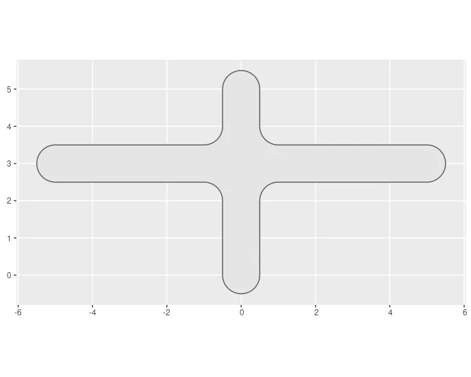
然而,Lovalery 关于线段端点准确性的观点提出了另一个好的问题。st_buffer 默认(ROUND)的 endCapStyle 会将线段长度扩展至缓冲区距离设置。
如果绘图限制截断所有街道末端,这是无关紧要的。如果街道的末端需要呈现在绘图中,则它们应该具有正确的长度。
更适当的缓冲设置是 endCapStyle = FLAT。请注意,当不匹配圆形线帽时,l2.smth 的平滑度设置从smoothness = 3 更改为smoothness = 0.2。

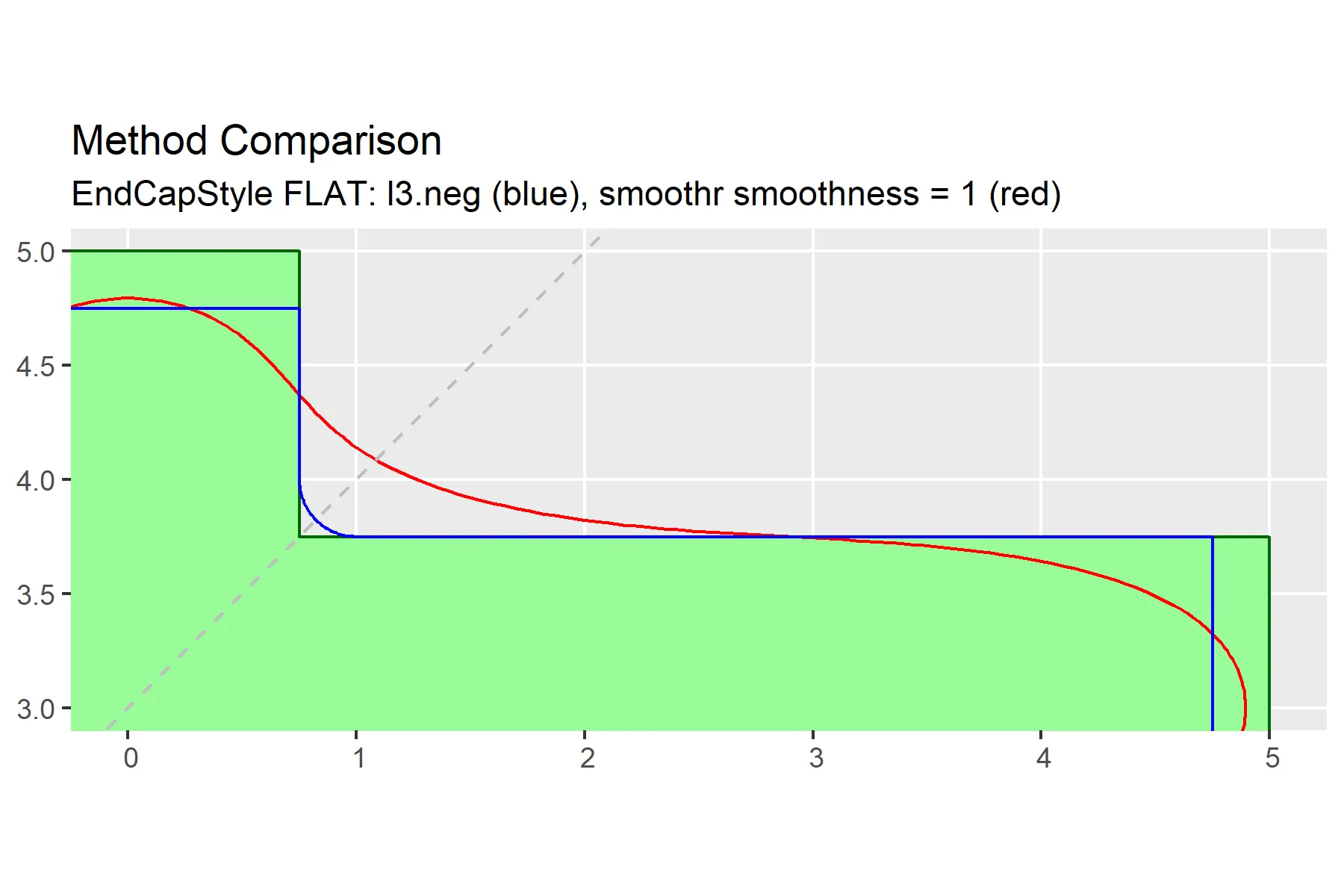
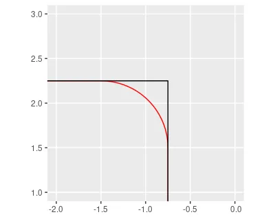
smoothr。最后,要挑剔一下,
smoothr提供的曲线不是对称的。平滑值越大,顶点长度之间的差异越大,则不对称性越明显。这是使用smoothness = 1的smoothr方法。
正如Lovalery所提到的,这取决于个体使用情况最好的选择。此外,普通观众是否会注意到街道比OSM说的短一米,或者曲线略微不对称?精度就像图形一样有趣...完美的精度可能并不重要,但它涉及到数学和数字,所以感觉应该很重要。
以上所有代码:
library(dplyr)
library(ggplot2)
library(sf)
library(smoothr)


l1 <- st_as_sfc(c("LINESTRING(0 0,0 5)","LINESTRING(-5 3,5 3)"))#,"LINESTRING(-5 7,5 7)"))
l2 <- l1 %>% st_union()

#### endCapStyle = ROUND ####

l2.base <- l2 %>% st_buffer(dist = 0.75, endCapStyle = "ROUND")
l2.neg <- l2 %>% st_buffer(dist = -0.25)
l2.smth <- l2 %>% smooth(method = "ksmooth", smoothness = 3, n= 50L)

l3 <- l1 %>% st_union %>% st_buffer(dist = 0.75+0.25, endCapStyle = "ROUND")
l3.neg <- st_buffer(l3, dist = -0.25)

ggplot()+
  geom_sf(data = l2.base, colour = "darkgreen", fill = "palegreen")+
  geom_sf(data = l2.neg, colour = "blue", fill = NA)+
  geom_sf(data = l2.smth, colour = "red", fill = NA)+
  geom_sf(data = l3.neg, colour = "cyan", fill = NA)+
  ggtitle("Method Comparison",
        subtitle = "EndCapStyle ROUND: l2 (green) v l2.smth (red), l2.neg (blue), l3.neg (cyan)") +
  scale_y_continuous(breaks = c(-1:6), limits = c(-1,6))+
  scale_x_continuous(breaks = c(-6:6), limits = c(-6,6))

#### endCapStyle = FLAT ####

l2.base <- l1 %>% st_union() %>% st_buffer(dist = 0.75, endCapStyle = "FLAT")
l2.neg <- l2.base %>% st_buffer(dist = -0.25)
l2.smth <- l2.base %>% smooth(method = "ksmooth", smoothness = 0.2, n= 50L)

l3 <- l1 %>% st_union %>% st_buffer(dist = 0.75+0.25, endCapStyle = "FLAT")
l3.neg <- st_buffer(l3, dist = -0.25)

ggplot()+
  geom_sf(data = l2.base, colour = "darkgreen", fill = "palegreen")+
  geom_sf(data = l2.neg, colour = "blue", fill = NA)+
  geom_sf(data = l2.smth, colour = "red", fill = NA)+
  geom_sf(data = l3.neg, colour = "cyan", fill = NA)+
  ggtitle("Method Comparison",
          subtitle = "EndCapStyle FLAT: l2 (green) v l2.smth (red), l2.neg (blue), l3.neg (cyan)") +
  scale_y_continuous(breaks = c(-1:6), limits = c(-1,6))+
  scale_x_continuous(breaks = c(-6:6), limits = c(-6,6))

#### illustrate asymmetry of smoothr method as l4.smth ####

l4.smth <- l2.base %>% smooth(method = "ksmooth", smoothness = 1, n= 50L)

ggplot()+
  geom_sf(data = l2.base, colour = "darkgreen", fill = "palegreen")+
  geom_sf(data = l4.smth, colour = "red", fill = NA)+
  geom_sf(data = l3.neg, colour = "blue", fill = NA)+
  geom_abline(slope = 1, intercept = 3, colour = "gray", linetype = "dashed")+
  ggtitle("Method Comparison",
          subtitle = "EndCapStyle FLAT: l3.neg (blue), smoothr smoothness = 1 (red)") +
  coord_sf(xlim = c(0,5), ylim = c(3,5))


st_buffer调用参数endCapStyle ='FLAT'或'SQUARE'。我很快会发布一篇编辑文章。 - mrhellmann