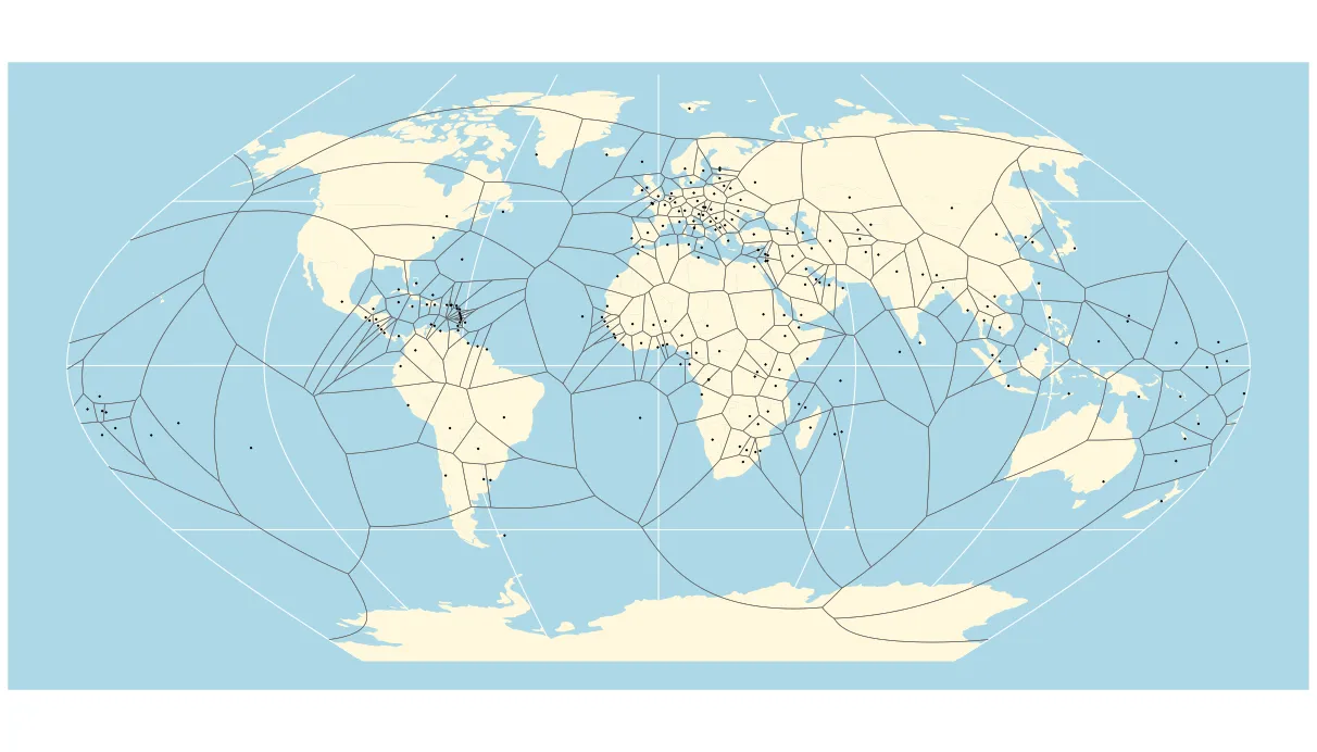
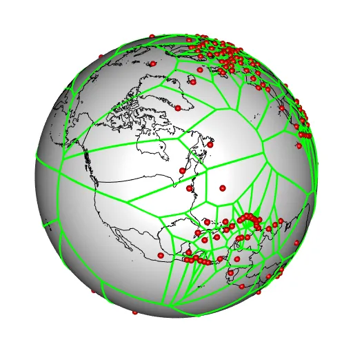
我希望用世界地图和 Voronoi 图案制作一个球形地图(不是它的投影),类似于 this using D3.js,但使用 R 语言。
据我所知(“Goodbye flat Earth, welcome S2 spherical geometry”),现在的
据我所知(“Goodbye flat Earth, welcome S2 spherical geometry”),现在的
sf 包完全基于 s2 包,应该能够满足我的需求。但我认为我没有得到预期的结果。以下是一个可重复的示例:library(tidyverse)
library(sf)
library(rnaturalearth)
library(tidygeocoder)
# just to be sure
sf::sf_use_s2(TRUE)
# download map
world_map <- rnaturalearth::ne_countries(
  scale = 'small',
  type = 'map_units',
  returnclass = 'sf')
# addresses that you want to find lat long and to become centroids of the voronoi tessellation
addresses <- tribble(
~addr,
"Juneau, Alaska" ,
"Saint Petersburg, Russia" ,
"Melbourne, Australia"
)
# retrive lat long using tidygeocoder
points <- addresses %>%
tidygeocoder::geocode(addr, method = 'osm')
# Transform lat long in a single geometry point and join with sf-base of the world
points <- points %>%
dplyr::rowwise() %>%
dplyr::mutate(point = list(sf::st_point(c(long, lat)))) %>%
sf::st_as_sf() %>%
sf::st_set_crs(4326)
# voronoi tessellation
voronoi <- sf::st_voronoi(sf::st_union( points ) ) %>%
sf::st_as_sf() %>%
sf::st_set_crs(4326)
# plot
ggplot2::ggplot() +
geom_sf(data = world_map,
mapping = aes(geometry = geometry),
fill = "gray95") +
geom_sf(data = points,
mapping = aes(geometry = point),
colour = "red") +
geom_sf(data = voronoi,
mapping = aes(geometry = x),
colour = "red",
alpha = 0.5)
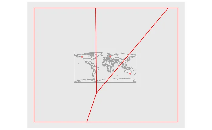
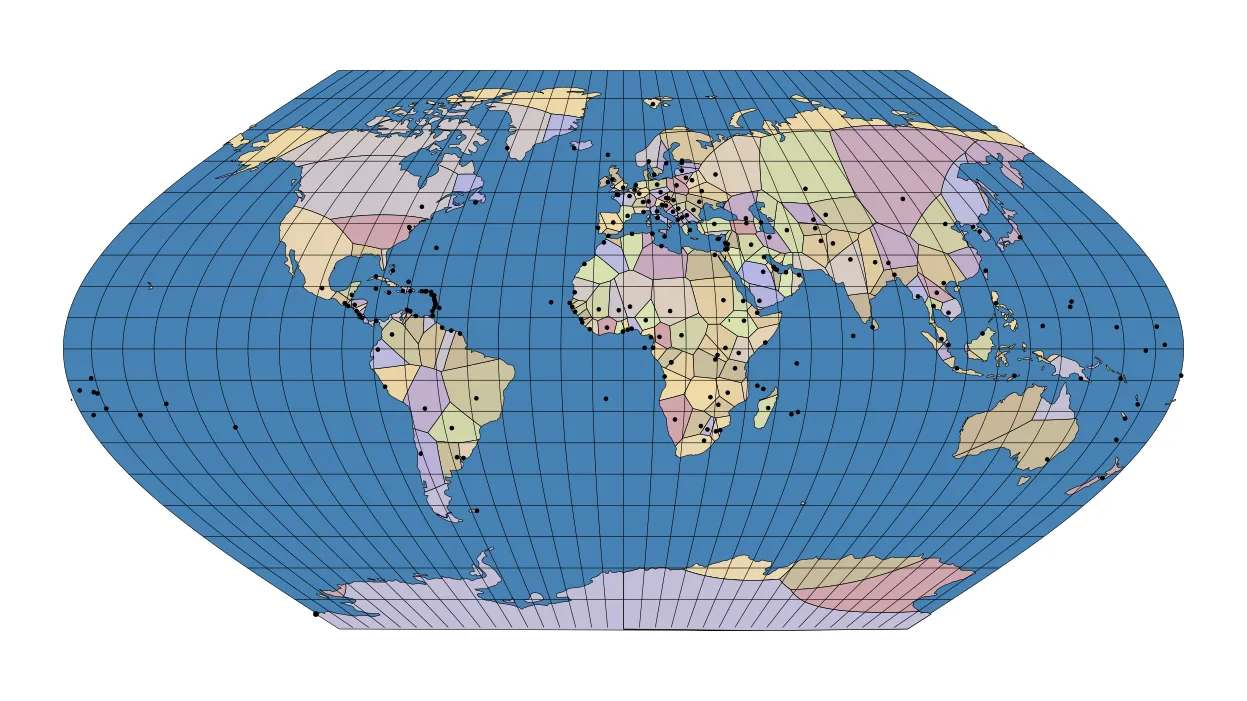
sf在球面上计算 Voronoi?