找出散点图中最密集区域的中心

Question

我有一组x和y坐标。 我想绘制它们并找出哪个区域具有密集的点。 我想找到该区域的中心坐标。

我编写了一个用于在x-y平面上绘制点的代码。

import numpy as np
import matplotlib.pyplot as plt
x = np.array([111,152,153,14,155,156,153,154,153,152,154,151,200,201,200])
y = np.array([112,151,153,12,153,154,155,153,152,153,152,153,202,202,204])
plt.scatter(x,y)
plt.show()

然而，我找不到密集绘制区域的中心。有人能帮帮我吗？

- Saankhya Mondal

---

首先定义“密集” - 你会包括哪个区域/邻域来计算一个区域的密度，以及什么是一个区域？你可以在每个点周围添加高斯函数并找到结果函数的最大值 - 但你必须先选择一个适当的半径。 - jbndlr

Answer 1

首先，您需要区分（并确定）密度和聚类。由于您的问题没有清晰地定义您所需的内容，因此我假设您想评估您的点中找到最大密度的位置。老实说，我很喜欢这个刺激性的任务，并选择了密度选项；）

单独使用术语“密度”是不充分的，因为有多种方法可以评估/估计/计算点云密度。我建议使用KDE（核密度估计器），因为它很容易适应自己的需求，并允许交换内核（方形、线性、高斯、余弦以及其他适用的内核）。

注意：完整代码如下；我现在将逐步介绍较小的片段。

准备工作

从您提供的点开始，以下代码段计算出您笛卡尔坐标系中的适当等间距网格。

RESOLUTION = 50
LOCALITY = 2.0

dx = max(pts_x) - min(pts_x)
dy = max(pts_y) - min(pts_y)

delta = min(dx, dy) / RESOLUTION
nx = int(dx / delta)
ny = int(dy / delta)
radius = (1 / LOCALITY) * min(dx, dy)

grid_x = np.linspace(min(pts_x), max(pts_x), num=nx)
grid_y = np.linspace(min(pts_y), max(pts_y), num=ny)

x, y = np.meshgrid(grid_x, grid_y)

你可以轻松地通过绘制plt.scatter（grid_x，grid_y）来检查它。 所有这些初步计算只是确保手头具有所有所需的值：我想能够指定某种分辨率和KDE内核扩展的局部性设置；此外，我们需要计算x和y方向上的最大点距离以进行网格生成，计算步幅delta，计算在x和y方向上的网格单元数，分别为nx和ny，以及根据我们的局部性设置计算内核半径。

内核密度估计

为了使用核函数估计点密度，如下代码段所述，我们确实需要两个函数。

def gauss(x1, x2, y1, y2):
    """
    Apply a Gaussian kernel estimation (2-sigma) to distance between points.

    Effectively, this applies a Gaussian kernel with a fixed radius to one
    of the points and evaluates it at the value of the euclidean distance
    between the two points (x1, y1) and (x2, y2).
    The Gaussian is transformed to roughly (!) yield 1.0 for distance 0 and
    have the 2-sigma located at radius distance.
    """
    return (
        (1.0 / (2.0 * math.pi))
        * math.exp(
            -1 * (3.0 * math.sqrt((x1 - x2)**2 + (y1 - y2)**2) / radius))**2
        / 0.4)


def _kde(x, y):
    """
    Estimate the kernel density at a given position.

    Simply sums up all the Gaussian kernel values towards all points
    (pts_x, pts_y) from position (x, y).
    """
    return sum([
        gauss(x, px, y, py)
        # math.sqrt((x - px)**2 + (y - py)**2)
        for px, py in zip(pts_x, pts_y)
    ])

第一个函数gauss同时执行两个任务：它使用由x1, x2, y1, y2定义的两个点计算它们的欧几里得距离，并使用该距离来评估高斯核函数值。当距离为0（或极小）时，高斯核经过变换近似为1.0，并且其2-sigma固定在先前计算的radius上。此特性由上述的locality设置控制。

识别最大值

幸运的是，numpy提供了一些不错的辅助函数，可以将任意Python函数应用于向量和矩阵上，因此计算就像下面这样简单：

kde = np.vectorize(_kde)  # Let numpy care for applying our kde to a vector
z = kde(x, y)

xi, yi = np.where(z == np.amax(z))
max_x = grid_x[xi][0]
max_y = grid_y[yi][0]
print(f"{max_x:.4f}, {max_y:.4f}")

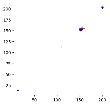
根据高斯核函数的设定和我的网格假设，您的情况下最大密度出现在：

155.2041, 154.0800

绘图

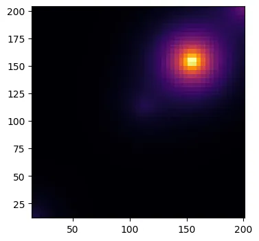
第一张图片展示了您的点云（蓝色十字）与识别出的最大值（红色十字）。第二张图片展示了使用第一个代码片段中的设置计算的高斯KDE估计密度。

完整代码

import math
import matplotlib.pyplot as plt
import numpy as np

pts_x = np.array([
    111, 152, 153, 14, 155, 156, 153, 154, 153, 152, 154, 151, 200, 201, 200])
pts_y = np.array([
    112, 151, 153, 12, 153, 154, 155, 153, 152, 153, 152, 153, 202, 202, 204])


RESOLUTION = 50
LOCALITY = 2.0

dx = max(pts_x) - min(pts_x)
dy = max(pts_y) - min(pts_y)

delta = min(dx, dy) / RESOLUTION
nx = int(dx / delta)
ny = int(dy / delta)
radius = (1 / LOCALITY) * min(dx, dy)

grid_x = np.linspace(min(pts_x), max(pts_x), num=nx)
grid_y = np.linspace(min(pts_y), max(pts_y), num=ny)

x, y = np.meshgrid(grid_x, grid_y)


def gauss(x1, x2, y1, y2):
    """
    Apply a Gaussian kernel estimation (2-sigma) to distance between points.

    Effectively, this applies a Gaussian kernel with a fixed radius to one
    of the points and evaluates it at the value of the euclidean distance
    between the two points (x1, y1) and (x2, y2).
    The Gaussian is transformed to roughly (!) yield 1.0 for distance 0 and
    have the 2-sigma located at radius distance.
    """
    return (
        (1.0 / (2.0 * math.pi))
        * math.exp(
            -1 * (3.0 * math.sqrt((x1 - x2)**2 + (y1 - y2)**2) / radius))**2
        / 0.4)


def _kde(x, y):
    """
    Estimate the kernel density at a given position.

    Simply sums up all the Gaussian kernel values towards all points
    (pts_x, pts_y) from position (x, y).
    """
    return sum([
        gauss(x, px, y, py)
        # math.sqrt((x - px)**2 + (y - py)**2)
        for px, py in zip(pts_x, pts_y)
    ])


kde = np.vectorize(_kde)  # Let numpy care for applying our kde to a vector
z = kde(x, y)

xi, yi = np.where(z == np.amax(z))
max_x = grid_x[xi][0]
max_y = grid_y[yi][0]
print(f"{max_x:.4f}, {max_y:.4f}")


fig, ax = plt.subplots()
ax.pcolormesh(x, y, z, cmap='inferno', vmin=np.min(z), vmax=np.max(z))
fig.set_size_inches(4, 4)
fig.savefig('density.png', bbox_inches='tight')

fig, ax = plt.subplots()
ax.scatter(pts_x, pts_y, marker='+', color='blue')
ax.scatter(grid_x[xi], grid_y[yi], marker='+', color='red', s=200)
fig.set_size_inches(4, 4)
fig.savefig('marked.png', bbox_inches='tight')

- jbndlr

---

好东西，为什么没有被批准呢？ - cincin21