Knitr & Beamer中的图层叠加问题

Question

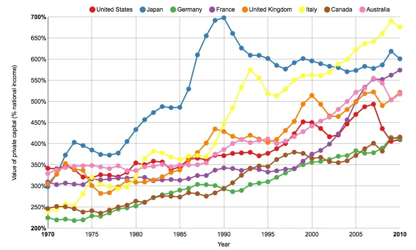
我正在创建一个beamer演示文稿，其中有一个图显示了几个时间序列和一个图例（比如10个国家的10个系列）。我想知道是否有一个相当简单的方法在beamer中动态地添加这些系列，可能是通过一块代码创建10张图像并将它们作为单独的帧依次插入。随着添加更多系列，图例也会更新。我猜想解决方案将涉及循环遍历包含10个国家的列表，逐个添加一个国家。

以下是一个相对精简的示例，显示了所有系列的单个图。我保留了原始数据，因此代码有点长，希望不会成为问题。[由于某种原因，图的引用编号没有显示出来，如果有人知道如何解决这个问题，我会相应更新代码。]

\documentclass{beamer}
\setbeamertemplate{navigation symbols}{}

<<setup, include=FALSE>>=
library(knitr)
### Load Libraries:
library(ggplot2)
library(scales)
library(xlsx)
library(reshape2)
library(RColorBrewer)
### Set Color & Shape Scheme:
colorPalette <- colorRampPalette(brewer.pal(9, "Set1"))(9)
shapePalette <- c(17, 2, 16, 1, 15, 0, 18, 5, 24)
### Load Data
df <- 
structure(list(Year = c(1970, 1971, 1972, 1973, 1974, 1975, 1976, 
1977, 1978, 1979, 1980, 1981, 1982, 1983, 1984, 1985, 1986, 1987, 
1988, 1989, 1990, 1991, 1992, 1993, 1994, 1995, 1996, 1997, 1998, 
1999, 2000, 2001, 2002, 2003, 2004, 2005, 2006, 2007, 2008, 2009, 
2010), US = c(3.42265371889757, 3.40883775035394, 3.48714154544623, 
3.3918808399871, 3.2149786413858, 3.19962742859596, 3.26773941561925, 
3.25691041518237, 3.21869258301295, 3.32930306011566, 3.54928091846329, 
3.50605987885847, 3.58930933604703, 3.56947109521563, 3.39111206142848, 
3.45519673484759, 3.63509892164379, 3.66190461652477, 3.62269304628001, 
3.72937652705034, 3.72194002526906, 3.77418488930653, 3.78624707450568, 
3.80047546800654, 3.71653349394787, 3.77606897480101, 3.88548730017041, 
4.00931412858258, 4.23951158932882, 4.52108993780641, 4.50347585611652, 
4.36449734409992, 4.1682991648011, 4.21151821995036, 4.47120525351423, 
4.69843213308901, 4.87750093832889, 4.94023200000774, 4.36016047791801, 
4.0607640596732, 4.09921895393402), Japan = c(2.9862145656143, 
3.27993801479434, 3.73480428038432, 4.03650790453792, 3.96024700378101, 
3.85535193733559, 3.74753619228984, 3.73415315599982, 3.78128411166629, 
4.05653721191352, 4.33699408182422, 4.57194662728378, 4.74070126950775, 
4.88225942346334, 4.85668276127374, 4.86434213335031, 5.29783056182241, 
6.106326266624, 6.55780181703131, 6.92283014250265, 6.98525270056026, 
6.61443218992994, 6.26683743354421, 6.09780509506938, 6.09430602943074, 
6.0205640302122, 5.85719231863445, 5.76982637280404, 5.92011081443946, 
6.01862462053832, 5.96279852951204, 5.89669397027792, 5.83636511534043, 
5.80547391655667, 5.7075874671511, 5.73828029065974, 5.83468446323163, 
5.78506098967758, 5.86809206830935, 6.19089593818452, 6.01237485111239
), Germany = c(2.25028311964994, 2.19997368560301, 2.2178393884591, 
2.18479912165755, 2.20126698092742, 2.29465431841867, 2.28676888070146, 
2.36449969898551, 2.45751763593208, 2.48603507321817, 2.5296440222246, 
2.62013228686627, 2.72744244161062, 2.79661246602516, 2.83672792160897, 
2.90342841424184, 2.94643285549051, 3.04244965338094, 3.03297460198842, 
3.01193899964686, 2.93337465632571, 2.86881455730272, 2.89751818871317, 
3.03685599967001, 3.07172228372608, 3.10277372448817, 3.20750040783546, 
3.31142434149651, 3.4068805122629, 3.50800500275626, 3.56473937826538, 
3.58484961640301, 3.63016879171539, 3.70546508418438, 3.7228401653644, 
3.83695092187362, 3.77789847916255, 3.79048630783758, 3.89654156987207, 
4.15195285079167, 4.11719616413334), France = c(3.10041308276844, 
3.03528473434106, 3.07224268696263, 3.04564643242234, 3.03367305451033, 
3.17046521393278, 3.14669782623641, 3.16669403005716, 3.18863871842954, 
3.18896735512728, 3.2118056113271, 3.20743980770504, 3.12834755391509, 
3.14710682768189, 3.15601383211585, 3.13941624302193, 3.17643343055692, 
3.24983758397325, 3.25067186123412, 3.37771667047246, 3.43020728196131, 
3.41686030175874, 3.37001936959952, 3.42404696480599, 3.39182912196306, 
3.33351776785474, 3.36339959767104, 3.40141917545778, 3.41654272775737, 
3.59046779724721, 3.75667824174458, 3.8453884378285, 3.99389592998013, 
4.23586045226769, 4.56786143701458, 4.99891524426584, 5.33816941234829, 
5.53459881682856, 5.52546980231239, 5.62610051047266, 5.74557817379884
), UK = c(3.05606066084056, 3.28136211640651, 3.53517285720912, 
3.4015466274181, 3.37355298562955, 3.01189577998554, 2.82778300365569, 
2.84264285305362, 2.98206660971185, 3.12871440091241, 3.09138672763463, 
3.09848424547132, 3.14369391882952, 3.22093566060216, 3.32453649939209, 
3.38203640523729, 3.60975706832705, 3.79175820721175, 4.01996620376656, 
4.35222485547853, 4.29074956516369, 4.17858265550709, 4.10601829597889, 
4.20374199691601, 4.11508157027746, 4.03388870700175, 4.10429676406955, 
4.31554950891114, 4.5334498290607, 4.93968597303074, 5.14555007361808, 
4.93640691154845, 4.65854702485502, 4.64802186851695, 4.81195849182541, 
4.99214720462646, 5.18939866500773, 5.22710830625107, 4.90522205950409, 
5.04405276332021, 5.21876019202926), Italy = c(2.39215637647118, 
2.44845609346066, 2.57763397859687, 2.5316735314333, 2.81963001666614, 
3.20731869907343, 3.04031888674008, 2.99802984507696, 2.9399636053426, 
2.98448248214816, 3.21914189644141, 3.6486889809305, 3.82528788673797, 
3.7839347408454, 3.68725754425826, 3.63013782782453, 3.71188604347889, 
3.72564825455312, 3.69103408796593, 4.01046564977317, 4.48058507188833, 
4.85343617432174, 5.34193146606732, 5.75157758748574, 5.55896964791881, 
5.18387020411741, 5.13555481434592, 5.2948199364687, 5.50848886386976, 
5.61393915207144, 5.63190988601601, 5.61666627489398, 5.69557515734195, 
5.88376044815484, 5.99564177268367, 6.2362241942999, 6.37208451589795, 
6.42483181625212, 6.60711186696451, 6.90849908711598, 6.76471157203947
), Canada = c(2.46999246515975, 2.51899440684339, 2.51072441779505, 
2.46367577973226, 2.38599551549661, 2.41613850112873, 2.35867265240764, 
2.43115439201043, 2.50563564378943, 2.54935677726461, 2.64401591844765, 
2.61476256582721, 2.72962132388488, 2.76836750499094, 2.76034296473846, 
2.74156887850989, 2.84357489511072, 2.82102192429222, 2.7618487567955, 
2.83942901661988, 2.94356263791855, 3.07986195414658, 3.25522196117649, 
3.40971743227054, 3.47667187371024, 3.46293485753507, 3.62994233169318, 
3.73637768424018, 3.80416175315756, 3.77481010019493, 3.65484296538209, 
3.68033672114661, 3.57770233271274, 3.55367989746207, 3.59965457056012, 
3.72599178459817, 3.88252681901122, 4.01544408308135, 3.82752126884386, 
4.12591287289822, 4.16188986951361), Australia = c(3.29797647418749, 
3.38491225540234, 3.44029047212715, 3.47125566425928, 3.4810218921083, 
3.48844677886234, 3.45360682034598, 3.41383660897562, 3.48141675382338, 
3.36482181389334, 3.37038861174626, 3.45350624176025, 3.46800728369306, 
3.51340651593045, 3.45348452180453, 3.49922503882649, 3.49995742217246, 
3.50727511525372, 3.55283382684878, 3.75439065549366, 3.86282026029909, 
4.00909028345048, 4.09888554022219, 4.03008779282658, 4.0786015030136, 
4.1171195564421, 4.00527485567151, 4.06619881966008, 4.17322264837539, 
4.2885540538951, 4.42376485715699, 4.53847634962058, 4.63205164187482, 
4.8161720868947, 5.00224755604537, 5.21903971255623, 5.3206272356995, 
5.55203639942649, 5.43848775952897, 5.03805394614743, 5.17911849231265
), Spain = c(NA, NA, NA, NA, NA, NA, NA, NA, NA, NA, NA, NA, 
NA, NA, NA, NA, NA, 3.61582686985211, 3.85335841950962, 4.15596177940659, 
4.34864142485489, 4.57079367080665, 4.52903738374002, 4.43043021221076, 
4.43875554480713, 4.29525396408518, 4.32973357345343, 4.32844261880396, 
4.42181465426299, 4.62656574873193, 4.78983037420811, 5.06749639036482, 
5.458653674397, 5.98283114191667, 6.65596447354794, 7.24210561415232, 
7.68573552177333, 7.92455000411218, 7.86235658455681, 7.8884251146486, 
7.55209874234684)), .Names = c("Year", "US", "Japan", "Germany", 
"France", "UK", "Italy", "Canada", "Australia", "Spain"), row.names = c(NA, 
-41L), class = "data.frame")
df <- melt(df, id.var = "Year")
names(df) <- c("Year","Country", "Percent")
@

\begin{document}
\title{Beamer `Overlay' with \texttt{knitr}}
\subtitle{1. Code overlays for each country data \\ 
2. Fix Figure reference not displaying}
\author{PatrickT based on Piketty}
\date{}

\maketitle

\begin{frame}[fragile]% need [fragile] option
\frametitle{Plot}
<<Figure1, fig.cap = '[Figure 5.3] http://piketty.pse.ens.fr/fr/capital21c', fig.height=4, fig.width=6, out.width='1\\maxwidth', dev='pdf', fig.align='center', cache=TRUE, warning=FALSE, echo=FALSE>>=
(p1 <- ggplot(data = df, aes(x = Year, y = Percent, group = Country, shape = Country, colour = Country)) + geom_line() + geom_point(aes(shape = Country, colour = Country), size = 3) + ylab("Value of private capital (% national income)") + xlab("") + theme_bw() + scale_y_continuous(labels = percent, breaks = pretty_breaks(n = 6)) + scale_x_continuous(breaks = seq(1970, 2010, by = 5)) + scale_shape_manual(name = "Country", values = shapePalette[1:9]) + scale_colour_manual(name = "Country", values = colorPalette[1:9]) + theme(legend.key = element_blank(), legend.position = c(.2, .75), legend.background = element_rect(colour = 'black')) + guides(shape = guide_legend(ncol = 2)))
@
\end{frame}

\end{document}

- PatrickT

---

这可能是有趣的：http://tex.stackexchange.com/questions/65096/how-to-make-a-diagram-composed-of-superimposed-layers-where-the-viewer-can-make - baptiste

Answer 1

我使用rCharts和nPlot结合nvd3/d3库创建了一个动态图。虽然这不是我想要的beamer/pdf方法，但对于我的目的来说还是令人满意的。

```{r 'Figure_5_3_rCharts',  message = FALSE, warning = FALSE, error = FALSE, echo = FALSE, tidy = FALSE, cache = FALSE}  
require(rCharts)
load("../../data/df_5_3.Rda") 
# round data for rChart tooltip display
df_5_3$value <- round(df_5_3$value, 3)
n <- nPlot(data = df_5_3, value ~ Year, group = 'variable', color = 'variable', shape = 'variable', type = 'lineChart') 
n$chart(forceY = c(2, 7))
n$yAxis(axisLabel = 'Value of private capital (% national income)')
n$chart(margin = list(left = 80)) 
n$yAxis(tickFormat = "#! function(d) {return Math.round(d*100*100)/100 + '%'} !#")
n$xAxis(axisLabel = 'Year')
n$chart(useInteractiveGuideline = TRUE)
n$chart(color = colorPalette)
n$addParams(height = 500, width = 800)
n$setTemplate(afterScript = '<style>
  .nv-point {
    stroke-opacity: 1!important;
    stroke-width: 5px!important;
    fill-opacity: 1!important;
  } 
</style>')
n$save('figures/Figure_5_3.html', standalone = TRUE)
```
<iframe src = 'figures/Figure_5_3.html' alt = "Figure 5.3. Private capital in rich countries, 1970-2010.">
</iframe><icaption class = 'icaption'>Figure 5.3. Private capital is worth between 2 and 3.5 years of national income in rich countries in 1970, and between 4 and 7 years of national income in 2010.</icaption>
<footer class = 'footnote'>  
Concept and data: Thomas Piketty. Chart created with ``rCharts`` (author: Ramnath Vaidyanathan)  
</footer> 

我在底部留了一些额外的代码片段，包括icaption和footer，以防有人觉得有用。这是一个截图：

- PatrickT