在绘制的数据和坐标轴之间去除空格

Question

我有以下数据框：

uniq <- structure(list(year = c(1986L, 1987L, 1991L, 1992L, 1993L, 1994L, 1995L, 1996L, 1997L, 1998L, 1999L, 2000L, 2001L, 2002L, 2003L, 2004L, 2005L, 2006L, 2007L, 2008L, 2009L, 2010L, 2011L, 2012L, 2013L, 2014L, 1986L, 1987L, 1991L, 1992L, 1993L, 1994L, 1995L, 1996L, 1997L, 1998L, 1999L, 2000L, 2001L, 2002L, 2003L, 2004L, 2005L, 2006L, 2007L, 2008L, 2009L, 2010L, 2011L, 2012L, 2013L, 2014L, 1986L, 1987L, 1991L, 1992L, 1993L, 1994L, 1995L, 1996L, 1997L, 1998L, 1999L, 2000L, 2001L, 2002L, 2003L, 2004L, 2005L, 2006L, 2007L, 2008L, 2009L, 2010L, 2011L, 2012L, 2013L, 2014L), uniq.loc = structure(c(1L, 1L, 1L, 1L, 1L, 1L, 1L, 1L, 1L, 1L, 1L, 1L, 1L, 1L, 1L, 1L, 1L, 1L, 1L, 1L, 1L, 1L, 1L, 1L, 1L, 1L, 2L, 2L, 2L, 2L, 2L, 2L, 2L, 2L, 2L, 2L, 2L, 2L, 2L, 2L, 2L, 2L, 2L, 2L, 2L, 2L, 2L, 2L, 2L, 2L, 2L, 2L, 3L, 3L, 3L, 3L, 3L, 3L, 3L, 3L, 3L, 3L, 3L, 3L, 3L, 3L, 3L, 3L, 3L, 3L, 3L, 3L, 3L, 3L, 3L, 3L, 3L, 3L), .Label = c("u.1", "u.2", "u.3"), class = "factor"), uniq.n = c(1, 1, 1, 2, 5, 4, 2, 16, 16, 10, 15, 14, 8, 12, 20, 11, 17, 30, 17, 21, 22, 19, 34, 44, 56, 11, 0, 0, 3, 3, 7, 17, 12, 21, 18, 10, 12, 9, 7, 11, 25, 14, 11, 17, 12, 24, 59, 17, 36, 50, 59, 12, 0, 0, 0, 1, 4, 6, 3, 3, 9, 3, 4, 2, 5, 2, 12, 6, 8, 8, 3, 2, 9, 5, 20, 7, 10, 8), uniq.p = c(100, 100, 25, 33.3, 31.2, 14.8, 11.8, 40, 37.2, 43.5, 48.4, 56, 40, 48, 35.1, 35.5, 47.2, 54.5, 53.1, 44.7, 24.4, 46.3, 37.8, 43.6, 44.8, 35.5, 0, 0, 75, 50, 43.8, 63, 70.6, 52.5, 41.9, 43.5, 38.7, 36, 35, 44, 43.9, 45.2, 30.6, 30.9, 37.5, 51.1, 65.6, 41.5, 40, 49.5, 47.2, 38.7, 0, 0, 0, 16.7, 25, 22.2, 17.6, 7.5, 20.9, 13, 12.9, 8, 25, 8, 21.1, 19.4, 22.2, 14.5, 9.4, 4.3, 10, 12.2, 22.2, 6.9, 8, 25.8)), .Names = c("year", "uniq.loc", "uniq.n", "uniq.p"), class = "data.frame", row.names = c(NA, -78L))

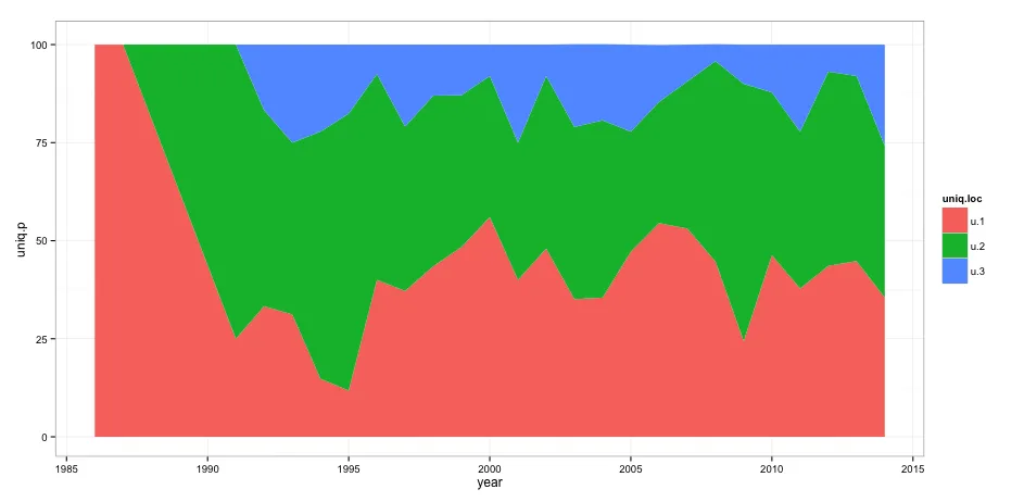
当我用以下方式制作面积图时：

ggplot(data = uniq) + 
  geom_area(aes(x = year, y = uniq.p, fill = uniq.loc), stat = "identity", position = "stack") +
  scale_x_continuous(limits=c(1986,2014)) +
  scale_y_continuous(limits=c(0,101)) +
  theme_bw()

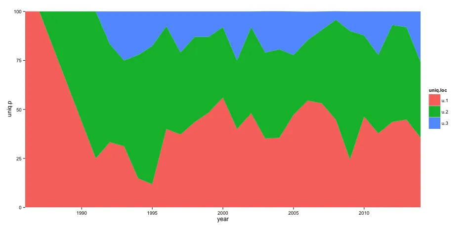
我得到了这个结果： 然而，我想要在轴和实际图形之间移除空白。当我添加 theme(panel.grid = element_blank(), panel.margin = unit(-0.8, "lines")) 时，我会收到以下错误信息：

Error in theme(panel.grid = element_blank(), panel.margin = unit(-0.8,  : 
  could not find function "unit"

有没有解决这个问题的建议？

- Jaap

---

我觉得你需要显式地加载grid包来使用unit。 - Tyler Rinker

@TylerRinker 谢谢！我不再收到错误消息了。我已经用另一种方法解决了这个问题，但这是一个很好的提醒，以后当我想设置边距时可以参考。 - Jaap

有时被称为紧凑布局。在这里提到这一点是为了让搜索引擎能够找到。 - anonymous

Answer 1

更新：请参见@divibisan的回答，以获取在最新版本的ggplot2中进一步的可能性。

---

从?scale_x_continuous关于expand参数的说明:

一组范围扩展常数，用于在数据周围添加一些填充，以确保它们与轴之间的距离足够远。默认情况下，对于连续变量，将比例扩大5％，对于离散变量，将每侧扩大0.6个单位。

因此，通过在scale_x_continuous和scale_y_continuous中添加expand = c(0,0)即可解决此问题。这也消除了添加panel.margin参数的需要。

代码：

ggplot(data = uniq) + 
  geom_area(aes(x = year, y = uniq.p, fill = uniq.loc), stat = "identity", position = "stack") +
  scale_x_continuous(limits = c(1986,2014), expand = c(0, 0)) +
  scale_y_continuous(limits = c(0,101), expand = c(0, 0)) +
  theme_bw() +
  theme(panel.grid = element_blank(),
        panel.border = element_blank())

结果为：

结果：

- Jaap

Answer 2

截至ggplot2版本3，有一个expand_scale()函数，您可以将其传递给expand=参数，以便为比例尺的每个侧面指定不同的扩展值。

从ggplot2版本3.3.0开始，expand_scale()已被弃用，推荐使用expansion，它的功能相同。

它还允许您选择扩展是绝对大小（使用add=参数）还是整个图形大小的百分比（使用mult=参数）：

ggplot(data = uniq) + 
  geom_area(aes(x = year, y = uniq.p, fill = uniq.loc), stat = "identity", position = "stack") +
  scale_x_continuous(limits = c(1986,2014), expand = c(0, 0)) +
  scale_y_continuous(limits = c(0,101), expand = expansion(mult = c(0, .1))) +
  theme_bw()

---

由于这是我获得最高票数的答案，所以我想扩展一下，更好地说明add=和mult=之间的区别。 两个选项都会将绘图区域在数据范围外特定数量的单位进行扩展。使用add时，通过绝对数量（以该轴使用的单位为单位）扩展该区域，而mult则通过指定该轴的总大小的比例来扩展该区域。

在下面的示例中，我使用add=10扩展底部，这将使绘图区域向下扩展10个单位到-10。 我使用mult=.15扩展顶部，这将使y轴上的数据的总大小的15％扩展到绘图区域的顶部。由于数据范围从0-100，因此为0.15 * 100 = 15个单位 - 因此它向上延伸到115。

ggplot(data = uniq) + 
    geom_area(aes(x = year, y = uniq.p, fill = uniq.loc),
              stat = "identity", position = "stack") +
    scale_x_continuous(limits = c(1986,2014), expand = c(0, 0)) +
    scale_y_continuous(limits = c(0,101),
                       breaks = seq(-10, 115, by=15),
                       expand = expansion(mult = c(0, .15),
                                          add = c(10, 0))) +
    theme_bw()

- divibisan

---

有没有办法从主题中删除扩展？我希望默认情况下它不存在（也许需要一个自定义的 scale_* 函数）。 - MokeEire

@MokeEire 我不知道有没有这样的功能。我认为你的想法是最好的：你可以定义一个自定义函数，它是带有这个默认设置的比例尺。 sxc <- function(...) scale_x_continuous(expand = expansion(add=0), ...)。然后你可以像使用scale_x_continuous一样使用sxc，甚至传入其他参数，但是具有该默认设置。 - divibisan

Answer 3

另一种产生相同结果的选择是使用 coord_cartesian 代替连续位置比例尺（x和y）：

ggplot(data = uniq) +  
  geom_area(aes(x = year, y = uniq.p, fill = uniq.loc), stat = "identity", position = "stack") +  
  coord_cartesian(xlim = c(1986,2014), ylim = c(0,101))+
  theme_bw() + theme(panel.grid=element_blank(), panel.border=element_blank())

- mpalanco

---

不错的替代方案，点赞。然而，如果您想指定间断点等内容，仍需要scales_x/y_continuous部分。 - Jaap

或者更简单的方法是按照@Marcus在此问题的评论中建议的，在coord_cartesian中设置expand = FALSE。 - tjebo

@Tjebo 输出结果略有不同，但实际上可能更接近于OP期望的结果。我稍后会将其添加到我的答案中。谢谢。 - mpalanco