原始问题
为什么一个循环比两个循环慢那么多?
结论:
案例1是一个经典的插值问题,但它是一个效率低下的问题。我认为这也是许多机器架构和开发人员最终建立和设计具有执行多线程应用程序以及并行编程能力的多核系统的主要原因之一。
从这种方法来看,不涉及硬件、操作系统和编译器如何协同工作来进行涉及RAM、缓存、页面文件等堆分配的数学计算,这些算法的基础告诉我们哪个解决方案更好。
我们可以使用一个比喻,将老板比作求和,代表必须在工人A和B之间移动的For Loop。
我们可以很容易地看出,由于工人之间需要旅行的距离和时间差异,
情况2至少比
情况1快一半以上。这个数学计算几乎完美地与
基准时间以及
装配指令的差异数量相吻合。
我现在将开始解释下面所有的工作原理。
评估问题
原帖中的代码:
const int n=100000;

for(int j=0;j<n;j++){
    a1[j] += b1[j];
    c1[j] += d1[j];
}
而且
for(int j=0;j<n;j++){
    a1[j] += b1[j];
}
for(int j=0;j<n;j++){
    c1[j] += d1[j];
}
考虑因素
考虑到原帖提出的有关两种变体for循环以及他后来修改的问题,涉及缓存行为的许多其他优秀答案和有用评论;我想在这里尝试通过不同的方式来处理这种情况和问题。
方法
考虑到两个循环以及有关缓存和页面文件的所有讨论,我想从不同的角度来看待这个问题。这种方法不涉及缓存和页面文件,也不涉及执行以分配内存,事实上,这种方法甚至不涉及实际硬件或软件。
视角
看了一段时间的代码后,问题和生成它的原因变得非常明显。让我们将其分解为算法问题,并从使用数学符号的角度来看待它,然后将类比应用于数学问题以及算法。
我们所知道的
我们知道这个循环将运行100,000次。我们也知道a1、b1、c1和d1是64位架构上的指针。在32位机器上的C++中,所有指针都是4字节,在64位机器上,它们的大小为8字节,因为指针具有固定长度。
我们知道我们有32字节可供分配,在两种情况下都是如此。唯一的区别是我们在每次迭代中分配32字节或两组2-8字节,在第二种情况下,我们为每个独立循环分配16字节的内存。
两个循环的总分配仍然相等,均为32字节。有了这些信息,让我们来展示这些概念的一般数学、算法和类比。
我们确实知道在两种情况下需要执行相同集合或组的操作的次数。我们确实知道在两种情况下需要分配的内存量。我们可以评估两种情况之间分配工作负载的整体工作量大致相同。
What We Don't Know
We do not know how long it will take for each case unless if we set a counter and run a benchmark test. However, the benchmarks were already included from the original question and from some of the answers and comments as well; and we can see a significant difference between the two and this is the whole reasoning for this proposal to this problem.
Let's Investigate
It is already apparent that many have already done this by looking at the heap allocations, benchmark tests, looking at RAM, cache, and page files. Looking at specific data points and specific iteration indices were also included and the various conversations about this specific problem have many people starting to question other related things about it. How do we begin to look at this problem by using mathematical algorithms and applying an analogy to it? We start off by making a couple of assertions! Then we build out our algorithm from there.
Our Assertions:
- We will let our loop and its iterations be a Summation that starts at 1 and ends at 100000 instead of starting with 0 as in the loops for we don't need to worry about the 0 indexing scheme of memory addressing since we are just interested in the algorithm itself.
- In both cases we have four functions to work with and two function calls with two operations being done on each function call. We will set these up as functions and calls to functions as the following:
F1(), F2(), f(a), f(b), f(c) and f(d).
The Algorithms:
1st Case: - Only one summation but two independent function calls.
Sum n=1 : [1,100000] = F1(), F2();
                       F1() = { f(a) = f(a) + f(b); }
                       F2() = { f(c) = f(c) + f(d); }
2nd Case: - Two summations but each has its own function call.
Sum1 n=1 : [1,100000] = F1();
                        F1() = { f(a) = f(a) + f(b); }

Sum2 n=1 : [1,100000] = F1();
                        F1() = { f(c) = f(c) + f(d); }
If you noticed F2() only exists in Sum from Case1 where F1() is contained in Sum from Case1 and in both Sum1 and Sum2 from Case2. This will be evident later on when we begin to conclude that there is an optimization that is happening within the second algorithm.
The iterations through the first case Sum calls f(a) that will add to its self f(b) then it calls f(c) that will do the same but add f(d) to itself for each 100000 iterations. In the second case, we have Sum1 and Sum2 that both act the same as if they were the same function being called twice in a row.
In this case we can treat Sum1 and Sum2 as just plain old Sum where Sum in this case looks like this: Sum n=1 : [1,100000] { f(a) = f(a) + f(b); } and now this looks like an optimization where we can just consider it to be the same function.
Summary with Analogy
With what we have seen in the second case it almost appears as if there is optimization since both for loops have the same exact signature, but this isn't the real issue. The issue isn't the work that is being done by f(a), f(b), f(c), and f(d). In both cases and the comparison between the two, it is the difference in the distance that the Summation has to travel in each case that gives you the difference in execution time.
Think of the for loops as being the summations that does the iterations as being a Boss that is giving orders to two people A & B and that their jobs are to meat C & D respectively and to pick up some package from them and return it. In this analogy, the for loops or summation iterations and condition checks themselves don't actually represent the Boss. What actually represents the Boss is not from the actual mathematical algorithms directly but from the actual concept of Scope and Code Block within a routine or subroutine, method, function, translation unit, etc. The first algorithm has one scope where the second algorithm has two consecutive scopes.
Within the first case on each call slip, the Boss goes to A and gives the order and A goes off to fetch B's package then the Boss goes to C and gives the orders to do the same and receive the package from D on each iteration.
Within the second case, the Boss works directly with A to go and fetch B's package until all packages are received. Then the Boss works with C to do the same for getting all of D's packages.
Since we are working with an 8-byte pointer and dealing with heap allocation let's consider the following problem. Let's say that the Boss is 100 feet from A and that A is 500 feet from C. We don't need to worry about how far the Boss is initially from C because of the order of executions. In both cases, the Boss initially travels from A first then to B. This analogy isn't to say that this distance is exact; it is just a useful test case scenario to show the workings of the algorithms.
In many cases when doing heap allocations and working with the cache and page files, these distances between address locations may not vary that much or they can vary significantly depending on the nature of the data types and the array sizes.
The Test Cases:
First Case: On first iteration the Boss has to initially go 100 feet to give the order slip to A and A goes off and does his thing, but then the Boss has to travel 500 feet to C to give him his order slip. Then on the next iteration and every other iteration after the Boss has to go back and forth 500 feet between the two.
Second Case: The Boss has to travel 100 feet on the first iteration to A, but after that, he is already there and just waits for A to get back until all slips are filled. Then the Boss has to travel 500 feet on the first iteration to C because C is 500 feet from A. Since this Boss( Summation, For Loop ) is being called right after working with A he then just waits there as he did with A until all of C's order slips are done.
The Difference In Distances Traveled
const n = 100000
distTraveledOfFirst = (100 + 500) + ((n-1)*(500 + 500))
// Simplify
distTraveledOfFirst = 600 + (99999*1000)
distTraveledOfFirst = 600 + 99999000
distTraveledOfFirst = 99999600
// Distance Traveled On First Algorithm = 99,999,600ft
distTraveledOfSecond = 100 + 500 = 600
// Distance Traveled On Second Algorithm = 600ft
The Comparison of Arbitrary Values
We can easily see that 600 is far less than approximately 100 million. Now, this isn't exact, because we don't know the actual difference in distance between which address of RAM or from which cache or page file each call on each iteration is going to be due to many other unseen variables. This is just an assessment of the situation to be aware of and looking at it from the worst-case scenario.
From these numbers it would almost appear as if algorithm one should be 99% slower than algorithm two; however, this is only the Boss's part or responsibility of the algorithms and it doesn't account for the actual workers A, B, C, & D and what they have to do on each and every iteration of the Loop. So the boss's job only accounts for about 15 - 40% of the total work being done. The bulk of the work that is done through the workers has a slightly bigger impact towards keeping the ratio of the speed rate differences to about 50-70%
The Observation: - The differences between the two algorithms
In this situation, it is the structure of the process of the work being done. It goes to show that Case 2 is more efficient from both the partial optimization of having a similar function declaration and definition where it is only the variables that differ by name and the distance traveled.
We also see that the total distance traveled in Case 1 is much farther than it is in Case 2 and we can consider this distance traveled our Time Factor between the two algorithms. Case 1 has considerable more work to do than Case 2 does.
This is observable from the evidence of the assembly instructions that were shown in both cases. Along with what was already stated about these cases, this doesn't account for the fact that in Case 1 the boss will have to wait for both A & C to get back before he can go back to A again for each iteration. It also doesn't account for the fact that if A or B is taking an extremely long time then both the Boss and the other worker(s) are idle waiting to be executed.
In Case 2 the only one being idle is the Boss until the worker gets back. So even this has an impact on the algorithm.
The OP's Amended Question(s)
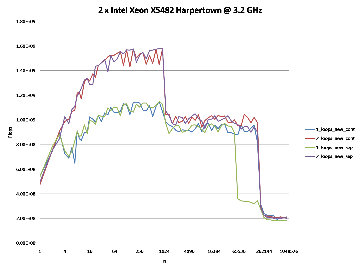
EDIT: The question turned out to be of no relevance, as the behavior severely depends on the sizes of the arrays (n) and the CPU cache. So if there is further interest, I rephrase the question:
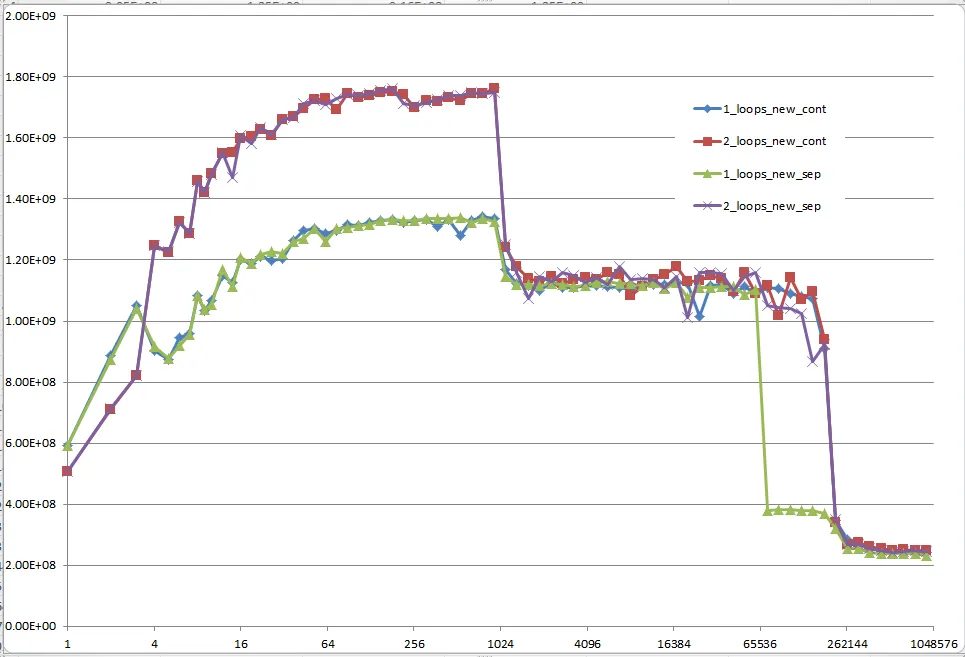
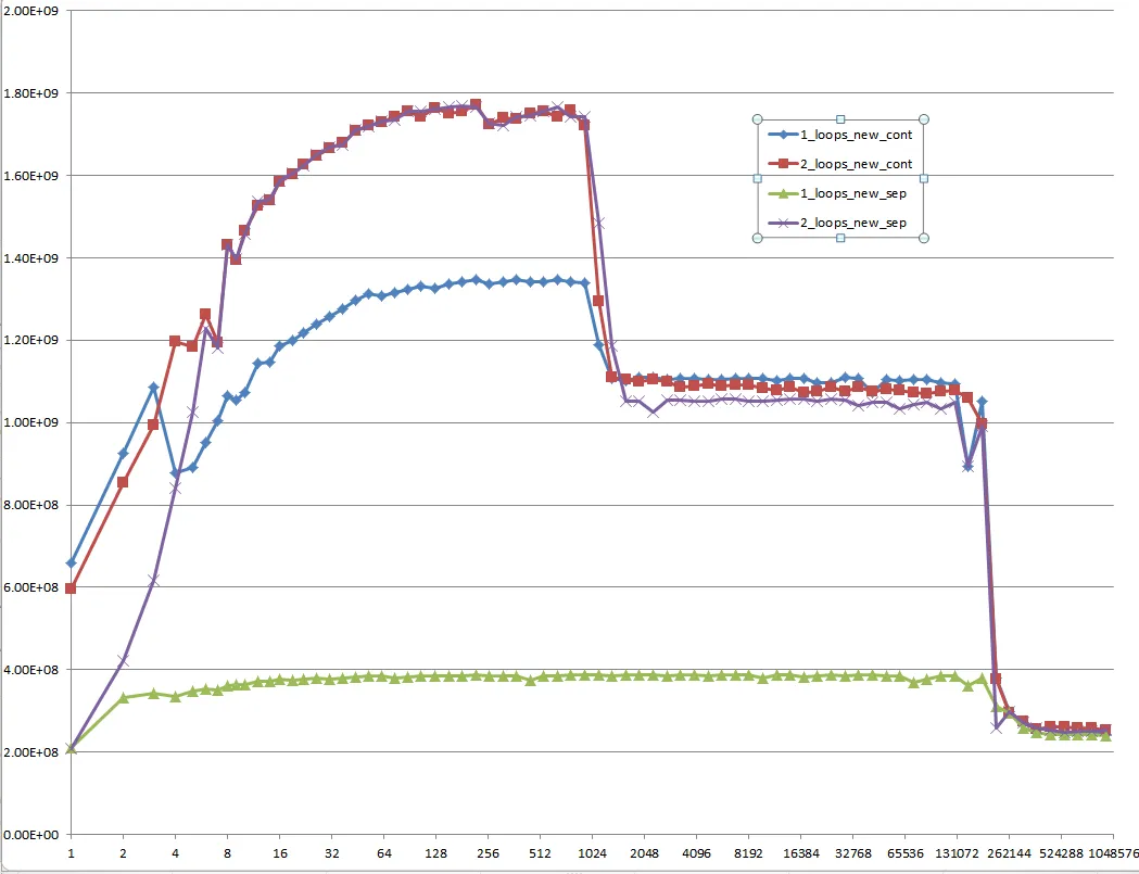
Could you provide some solid insight into the details that lead to the different cache behaviors as illustrated by the five regions on the following graph?
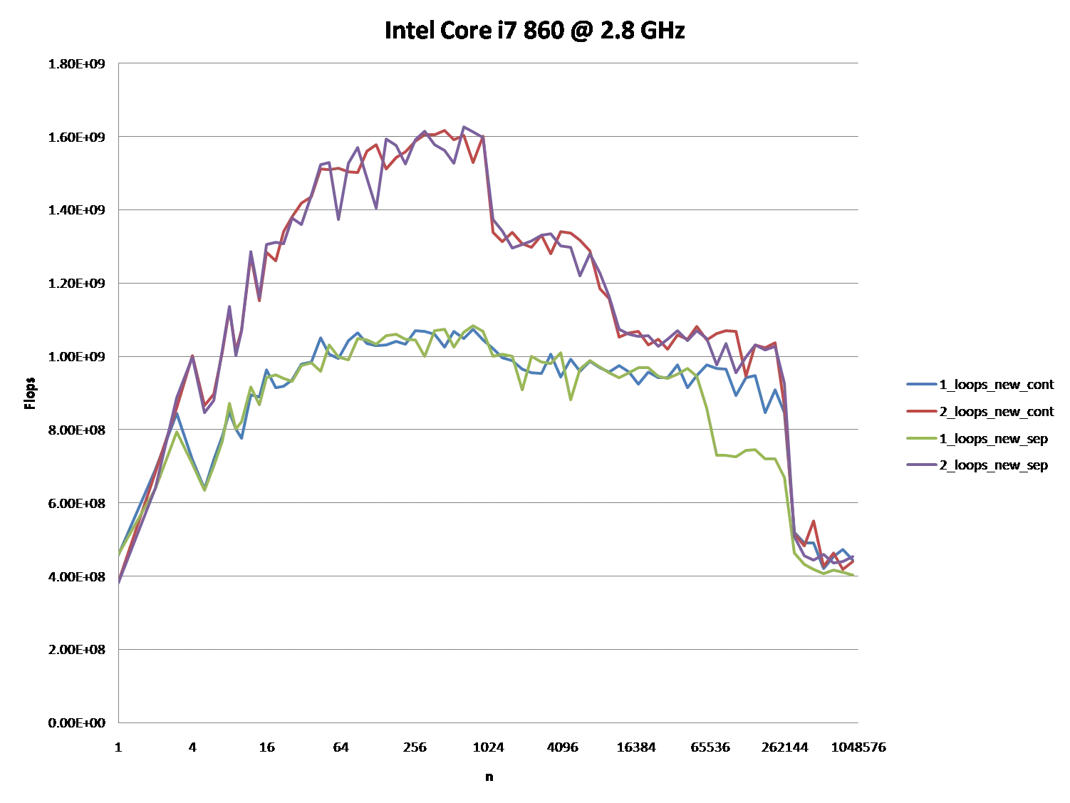
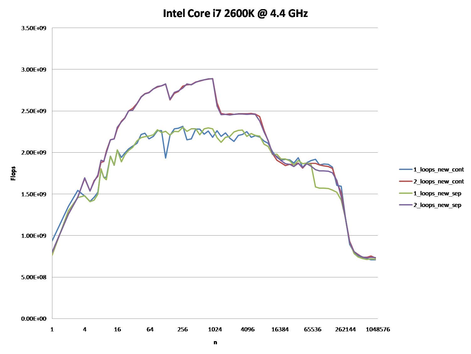
It might also be interesting to point out the differences between CPU/cache architectures, by providing a similar graph for these CPUs.
Regarding These Questions
As I have demonstrated without a doubt, there is an underlying issue even before the Hardware and Software becomes involved.
Now as for the management of memory and caching along with page files, etc. which all work together in an integrated set of systems between the following:
- The architecture (hardware, firmware, some embedded drivers, kernels and assembly instruction sets).
- The OS (file and memory management systems, drivers and the registry).
- The compiler (translation units and optimizations of the source code).
- And even the source code itself with its set(s) of distinctive algorithms.
We can already see that there is a bottleneck that is happening within the first algorithm before we even apply it to any machine with any arbitrary architecture, OS, and programmable language compared to the second algorithm. There already existed a problem before involving the intrinsics of a modern computer.
The Ending Results
However; it is not to say that these new questions are not of importance because they themselves are and they do play a role after all. They do impact the procedures and the overall performance and that is evident with the various graphs and assessments from many who have given their answer(s) and or comment(s).
If you paid attention to the analogy of the Boss and the two workers A & B who had to go and retrieve packages from C & D respectively and considering the mathematical notations of the two algorithms in question; you can see without the involvement of the computer hardware and software Case 2 is approximately 60% faster than Case 1.
When you look at the graphs and charts after these algorithms have been applied to some source code, compiled, optimized, and executed through the OS to perform their operations on a given piece of hardware, you can even see a little more degradation between the differences in these algorithms.
If the Data set is fairly small it may not seem all that bad of a difference at first. However, since Case 1 is about 60 - 70% slower than Case 2 we can look at the growth of this function in terms of the differences in time executions:
DeltaTimeDifference approximately = Loop1(time) - Loop2(time)
//where
Loop1(time) = Loop2(time) + (Loop2(time)*[0.6,0.7]) // approximately
// So when we substitute this back into the difference equation we end up with
DeltaTimeDifference approximately = (Loop2(time) + (Loop2(time)*[0.6,0.7])) - Loop2(time)
// And finally we can simplify this to
DeltaTimeDifference approximately = [0.6,0.7]*Loop2(time)
This approximation is the average difference between these two loops both algorithmically and machine operations involving software optimizations and machine instructions.
When the data set grows linearly, so does the difference in time between the two. Algorithm 1 has more fetches than algorithm 2 which is evident when the Boss has to travel back and forth the maximum distance between A & C for every iteration after the first iteration while algorithm 2 the Boss has to travel to A once and then after being done with A he has to travel a maximum distance only one time when going from A to C.
Trying to have the Boss focusing on doing two similar things at once and juggling them back and forth instead of focusing on similar consecutive tasks is going to make him quite angry by the end of the day since he had to travel and work twice as much. Therefore do not lose the scope of the situation by letting your boss getting into an interpolated bottleneck because the boss's spouse and children wouldn't appreciate it.
Amendment: Software Engineering Design Principles
-- The difference between local Stack and heap allocated computations within iterative for loops and the difference between their usages, their efficiencies, and effectiveness --
The mathematical algorithm that I proposed above mainly applies to loops that perform operations on data that is allocated on the heap.
- Consecutive Stack Operations:
- If the loops are performing operations on data locally within a single code block or scope that is within the stack frame it will still sort of apply, but the memory locations are much closer where they are typically sequential and the difference in distance traveled or execution time is almost negligible. Since there are no allocations being done within the heap, the memory isn't scattered, and the memory isn't being fetched through ram. The memory is typically sequential and relative to the stack frame and stack pointer.
- When consecutive operations are being done on the stack, a modern processor will cache repetitive values and addresses keeping these values within local cache registers. The time of operations or instructions here is on the order of nano-seconds.
- Consecutive Heap Allocated Operations:
- When you begin to apply heap allocations and the processor has to fetch the memory addresses on consecutive calls, depending on the architecture of the CPU, the bus controller, and the RAM modules the time of operations or execution can be on the order of micro to milliseconds. In comparison to cached stack operations, these are quite slow.
- The CPU will have to fetch the memory address from RAM and typically anything across the system bus is slow compared to the internal data paths or data buses within the CPU itself.
So when you are working with data that needs to be on the heap and you are traversing through them in loops, it is more efficient to keep each data set and its corresponding algorithms within its own single loop. You will get better optimizations compared to trying to factor out consecutive loops by putting multiple operations of different data sets that are on the heap into a single loop.
It is okay to do this with data that is on the stack since they are frequently cached, but not for data that has to have its memory address queried every iteration.
This is where software engineering and software architecture design comes into play. It is the ability to know how to organize your data, knowing when to cache your data, knowing when to allocate your data on the heap, knowing how to design and implement your algorithms, and knowing when and where to call them.
You might have the same algorithm that pertains to the same data set, but you might want one implementation design for its stack variant and another for its heap-allocated variant just because of the above issue that is seen from its O(n) complexity of the algorithm when working with the heap.
From what I've noticed over the years, many people do not take this fact into consideration. They will tend to design one algorithm that works on a particular data set and they will use it regardless of the data set being locally cached on the stack or if it was allocated on the heap.
If you want true optimization, yes it might seem like code duplication, but to generalize it would be more efficient to have two variants of the same algorithm. One for stack operations, and the other for heap operations that are performed in iterative loops!
Here's a pseudo example: Two simple structs, one algorithm.
struct A {
int data;
A() : data{0}{}
A(int a) : data{a}{}
};
struct B {
int data;
B() : data{0}{}
A(int b) : data{b}{}
}
template<typename T>
void Foo( T& t ) {
}
A dataSetA[10] = {};
B dataSetB[10] = {};
for (int i = 0; i < 10; i++ ) {
Foo(dataSetA[i]);
Foo(dataSetB[i]);
}
A* dataSetA = new [] A();
B* dataSetB = new [] B();
for ( int i = 0; i < 10; i++ ) {
Foo(dataSetA[i]);
Foo(dataSetB[i]);
}
for (int i = 0; i < 10; i++ ) {
Foo(dataSetA[i]);
}
for (int i = 0; i < 10; i++ ) {
Foo(dataSetB[i]);
}
This is what I was referring to by having separate implementations for stack variants versus heap variants. The algorithms themselves don't matter too much, it's the looping structures that you will use them in that do.

d1[j]可能与a1[j]产生别名,因此编译器可能会放弃执行某些内存优化。然而,如果将写入内存分为两个循环,就不会发生这种情况。 - rturradoL1D、L1D_CACHE_ST、L2_RQSTS和L2_DATA_RQSTS性能计数器会很有启示性。请参见Intel Core i7(Nehalem)事件。 - jww