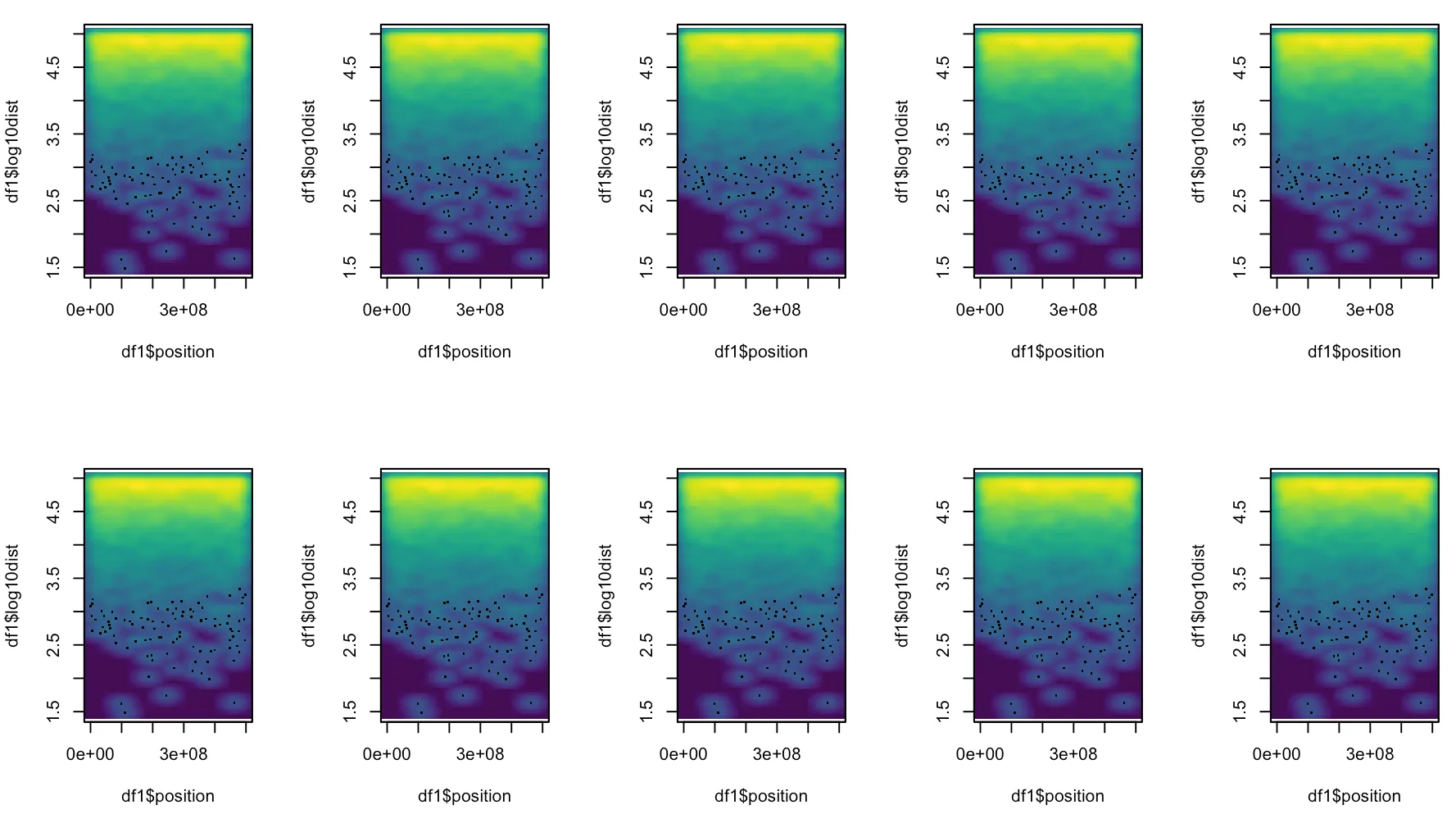
有人知道如何创建像屏幕截图中那样的图形吗? 我尝试通过调整alpha来获得类似的效果,但这将使异常值几乎不可见。 我只从一个叫做FlowJo的软件中了解到这种类型的图表,他们称之为“伪彩色点图”。 不确定这是否是正式术语。
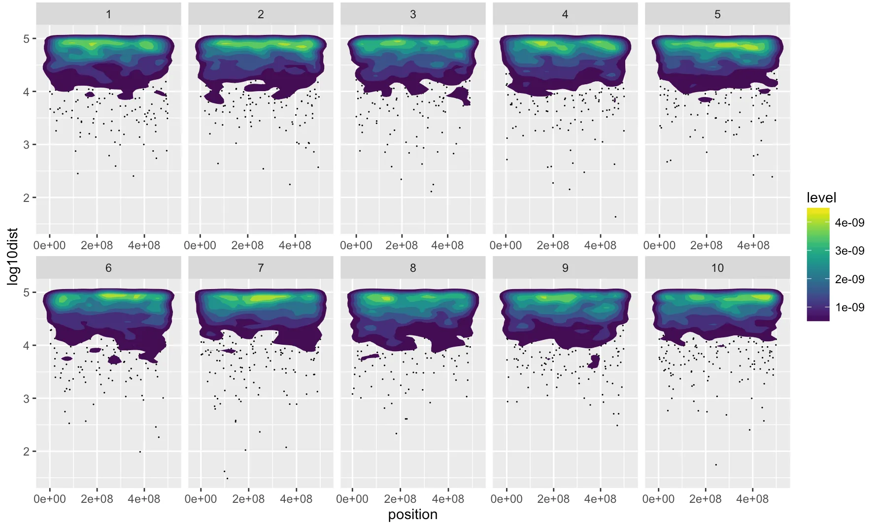
我想在ggplot2中特别完成它,因为我需要分面选项。 我附上了另一张我的图表的屏幕快照。 垂直线表示某些基因组区域的突变簇。 其中一些簇比其他簇密集得多。 我想使用密度颜色来说明这一点。
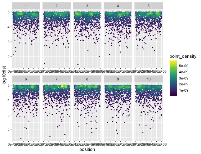
数据很大且难以模拟,但这里有一次尝试。 它看起来与实际数据不同,但数据格式相同。
我想在ggplot2中特别完成它,因为我需要分面选项。 我附上了另一张我的图表的屏幕快照。 垂直线表示某些基因组区域的突变簇。 其中一些簇比其他簇密集得多。 我想使用密度颜色来说明这一点。
数据很大且难以模拟,但这里有一次尝试。 它看起来与实际数据不同,但数据格式相同。
chr <- c(rep(1:10,1000))
position <- runif(10000, min=0, max=5e8)
distance <- runif(10000, min=1, max=1e5)
log10dist <- log10(distance)

df1 <- data.frame(chr, position, distance, log10dist)

ggplot(df1, aes(position, log10dist)) +
  geom_point(shape=16, size=0.25, alpha=0.5, show.legend = FALSE) +
  facet_wrap(~chr, ncol = 5, nrow = 2, scales = "free_x")
非常感谢您的帮助。
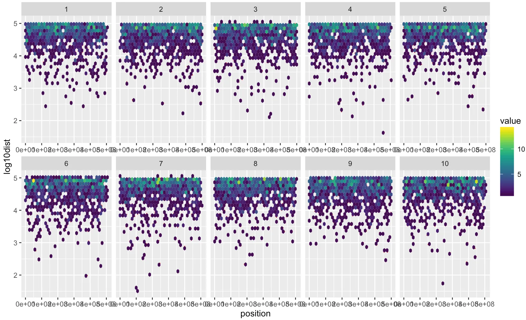
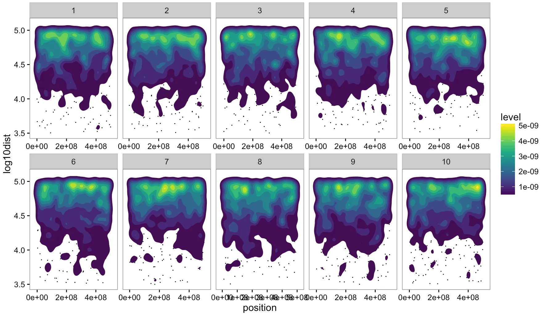
geom_hex。 - RolandsmoothScatter()调用(通过grDevices:::.smoothScatterCalcDensity())KernSmooth::bkde2D()然后过滤掉非异常值。您可以使用ggalt::geom_bkde2d()进行密度图绘制,并在其下方绘制geom_point()。您没有提供任何数据供其他人模拟。 - hrbrmstrgeom_bkde2D()似乎并没有给我想要的结果。也许我必须尝试smoothScatter,并将单个染色体粘贴在一页上以获得分面效果。我还会尝试使用hexbin。让我们看看。 - Peer Wünsche