我想我找到了解决这个问题的答案。但我仍希望得到帮助,让代码更加简洁 - 你可以看到我复制了很多内容。
mtcars_mpg_wt <- mtcars %>%
select(mpg, wt)
boots <- bootstraps(mtcars_mpg_wt, times = 250, apparent = TRUE)
boots
fit_nls_on_bootstrap <- function(split) {
lm(mpg ~ wt, analysis(split))
}
library(purrr)
boot_models <-
boots %>%
dplyr::mutate(model = map(splits, fit_nls_on_bootstrap),
coef_info = map(model, tidy))
boot_coefs <-
boot_models %>%
unnest(coef_info)
percentile_intervals <- int_pctl(boot_models, coef_info)
percentile_intervals
ggplot(boot_coefs, aes(estimate)) +
geom_histogram(bins = 30) +
facet_wrap( ~ term, scales = "free") +
labs(title="", subtitle = "mpg ~ wt - Linear Regression Bootstrap Resampling") +
theme(plot.title = element_text(hjust = 0.5, face = "bold")) +
theme(plot.subtitle = element_text(hjust = 0.5)) +
labs(caption = "95% Confidence Interval Parameter Estimates, Intercept + Estimate") +
geom_vline(aes(xintercept = .lower), data = percentile_intervals, col = "blue") +
geom_vline(aes(xintercept = .upper), data = percentile_intervals, col = "blue")
boot_aug <-
boot_models %>%
sample_n(50) %>%
mutate(augmented = map(model, augment)) %>%
unnest(augmented)
glimpse(boot_aug)
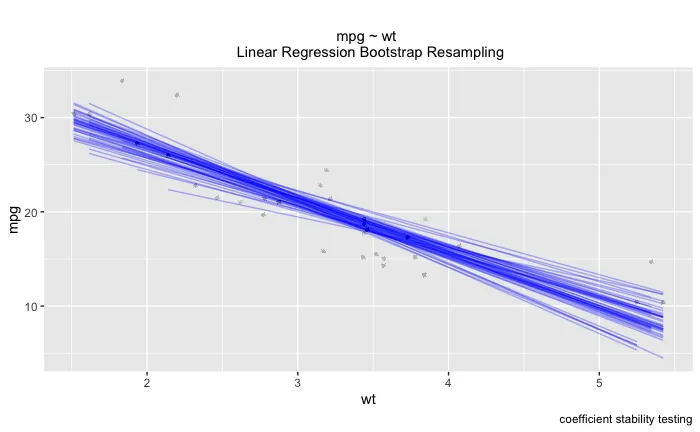
ggplot(boot_aug, aes(wt, mpg)) +
geom_line(aes(y = .fitted, group = id), alpha = .3, col = "blue") +
geom_point(alpha = 0.005) +
labs(title="", subtitle = "mpg ~ wt \n Linear Regression Bootstrap Resampling") +
theme(plot.title = element_text(hjust = 0.5, face = "bold")) +
theme(plot.subtitle = element_text(hjust = 0.5)) +
labs(caption = "coefficient stability testing")
boot_aug_1 <- boot_aug %>%
mutate(factor = "wt")
mtcars_mpg_disp <- mtcars %>%
select(mpg, disp)
boots <- bootstraps(mtcars_mpg_disp, times = 250, apparent = TRUE)
boots
fit_nls_on_bootstrap <- function(split) {
lm(mpg ~ disp, analysis(split))
}
library(purrr)
boot_models <-
boots %>%
dplyr::mutate(model = map(splits, fit_nls_on_bootstrap),
coef_info = map(model, tidy))
boot_coefs <-
boot_models %>%
unnest(coef_info)
percentile_intervals <- int_pctl(boot_models, coef_info)
percentile_intervals
ggplot(boot_coefs, aes(estimate)) +
geom_histogram(bins = 30) +
facet_wrap( ~ term, scales = "free") +
labs(title="", subtitle = "mpg ~ wt - Linear Regression Bootstrap Resampling") +
theme(plot.title = element_text(hjust = 0.5, face = "bold")) +
theme(plot.subtitle = element_text(hjust = 0.5)) +
labs(caption = "95% Confidence Interval Parameter Estimates, Intercept + Estimate") +
geom_vline(aes(xintercept = .lower), data = percentile_intervals, col = "blue") +
geom_vline(aes(xintercept = .upper), data = percentile_intervals, col = "blue")
boot_aug <-
boot_models %>%
sample_n(50) %>%
mutate(augmented = map(model, augment)) %>%
unnest(augmented)
glimpse(boot_aug)
ggplot(boot_aug, aes(disp, mpg)) +
geom_line(aes(y = .fitted, group = id), alpha = .3, col = "blue") +
geom_point(alpha = 0.005) +
labs(title="", subtitle = "mpg ~ disp \n Linear Regression Bootstrap Resampling") +
theme(plot.title = element_text(hjust = 0.5, face = "bold")) +
theme(plot.subtitle = element_text(hjust = 0.5)) +
labs(caption = "coefficient stability testing")
boot_aug_2 <- boot_aug %>%
mutate(factor = "disp")
mtcars_mpg_drat <- mtcars %>%
select(mpg, drat)
boots <- bootstraps(mtcars_mpg_drat, times = 250, apparent = TRUE)
boots
fit_nls_on_bootstrap <- function(split) {
lm(mpg ~ drat, analysis(split))
}
library(purrr)
boot_models <-
boots %>%
dplyr::mutate(model = map(splits, fit_nls_on_bootstrap),
coef_info = map(model, tidy))
boot_coefs <-
boot_models %>%
unnest(coef_info)
percentile_intervals <- int_pctl(boot_models, coef_info)
percentile_intervals
ggplot(boot_coefs, aes(estimate)) +
geom_histogram(bins = 30) +
facet_wrap( ~ term, scales = "free") +
labs(title="", subtitle = "mpg ~ wt - Linear Regression Bootstrap Resampling") +
theme(plot.title = element_text(hjust = 0.5, face = "bold")) +
theme(plot.subtitle = element_text(hjust = 0.5)) +
labs(caption = "95% Confidence Interval Parameter Estimates, Intercept + Estimate") +
geom_vline(aes(xintercept = .lower), data = percentile_intervals, col = "blue") +
geom_vline(aes(xintercept = .upper), data = percentile_intervals, col = "blue")
boot_aug <-
boot_models %>%
sample_n(50) %>%
mutate(augmented = map(model, augment)) %>%
unnest(augmented)
glimpse(boot_aug)
ggplot(boot_aug, aes(drat, mpg)) +
geom_line(aes(y = .fitted, group = id), alpha = .3, col = "blue") +
geom_point(alpha = 0.005) +
labs(title="", subtitle = "mpg ~ wt \n Linear Regression Bootstrap Resampling") +
theme(plot.title = element_text(hjust = 0.5, face = "bold")) +
theme(plot.subtitle = element_text(hjust = 0.5)) +
labs(caption = "coefficient stability testing")
boot_aug_3 <- boot_aug %>%
mutate(factor = "drat")
mtcars_mpg_hp <- mtcars %>%
select(mpg, hp)
boots <- bootstraps(mtcars_mpg_hp, times = 250, apparent = TRUE)
boots
fit_nls_on_bootstrap <- function(split) {
lm(mpg ~ hp, analysis(split))
}
library(purrr)
boot_models <-
boots %>%
dplyr::mutate(model = map(splits, fit_nls_on_bootstrap),
coef_info = map(model, tidy))
boot_coefs <-
boot_models %>%
unnest(coef_info)
percentile_intervals <- int_pctl(boot_models, coef_info)
percentile_intervals
ggplot(boot_coefs, aes(estimate)) +
geom_histogram(bins = 30) +
facet_wrap( ~ term, scales = "free") +
labs(title="", subtitle = "mpg ~ wt - Linear Regression Bootstrap Resampling") +
theme(plot.title = element_text(hjust = 0.5, face = "bold")) +
theme(plot.subtitle = element_text(hjust = 0.5)) +
labs(caption = "95% Confidence Interval Parameter Estimates, Intercept + Estimate") +
geom_vline(aes(xintercept = .lower), data = percentile_intervals, col = "blue") +
geom_vline(aes(xintercept = .upper), data = percentile_intervals, col = "blue")
boot_aug <-
boot_models %>%
sample_n(50) %>%
mutate(augmented = map(model, augment)) %>%
unnest(augmented)
glimpse(boot_aug)
ggplot(boot_aug, aes(hp, mpg)) +
geom_line(aes(y = .fitted, group = id), alpha = .3, col = "blue") +
geom_point(alpha = 0.005) +
labs(title="", subtitle = "mpg ~ wt \n Linear Regression Bootstrap Resampling") +
theme(plot.title = element_text(hjust = 0.5, face = "bold")) +
theme(plot.subtitle = element_text(hjust = 0.5)) +
labs(caption = "coefficient stability testing")
boot_aug_4 <- boot_aug %>%
mutate(factor = "hp")
mtcars_mpg_qsec <- mtcars %>%
select(mpg, qsec)
boots <- bootstraps(mtcars_mpg_qsec, times = 250, apparent = TRUE)
boots
fit_nls_on_bootstrap <- function(split) {
lm(mpg ~ qsec, analysis(split))
}
library(purrr)
boot_models <-
boots %>%
dplyr::mutate(model = map(splits, fit_nls_on_bootstrap),
coef_info = map(model, tidy))
boot_coefs <-
boot_models %>%
unnest(coef_info)
percentile_intervals <- int_pctl(boot_models, coef_info)
percentile_intervals
ggplot(boot_coefs, aes(estimate)) +
geom_histogram(bins = 30) +
facet_wrap( ~ term, scales = "free") +
labs(title="", subtitle = "mpg ~ wt - Linear Regression Bootstrap Resampling") +
theme(plot.title = element_text(hjust = 0.5, face = "bold")) +
theme(plot.subtitle = element_text(hjust = 0.5)) +
labs(caption = "95% Confidence Interval Parameter Estimates, Intercept + Estimate") +
geom_vline(aes(xintercept = .lower), data = percentile_intervals, col = "blue") +
geom_vline(aes(xintercept = .upper), data = percentile_intervals, col = "blue")
boot_aug <-
boot_models %>%
sample_n(50) %>%
mutate(augmented = map(model, augment)) %>%
unnest(augmented)
glimpse(boot_aug)
ggplot(boot_aug, aes(qsec, mpg)) +
geom_line(aes(y = .fitted, group = id), alpha = .3, col = "blue") +
geom_point(alpha = 0.005) +
labs(title="", subtitle = "mpg ~ wt \n Linear Regression Bootstrap Resampling") +
theme(plot.title = element_text(hjust = 0.5, face = "bold")) +
theme(plot.subtitle = element_text(hjust = 0.5)) +
labs(caption = "coefficient stability testing")
boot_aug_5 <- boot_aug %>%
mutate(factor = "qsec")
boot_aug_total <- bind_rows(boot_aug_1, boot_aug_2, boot_aug_3, boot_aug_4, boot_aug_5)
boot_aug_total <- boot_aug_total %>%
select(disp, drat, hp, qsec, wt, mpg, .fitted, id, factor)
boot_aug_total_2 <- pivot_longer(boot_aug_total, names_to = 'names', values_to = 'values', 1:5)
boot_aug_total_2 <- boot_aug_total_2 %>%
drop_na()
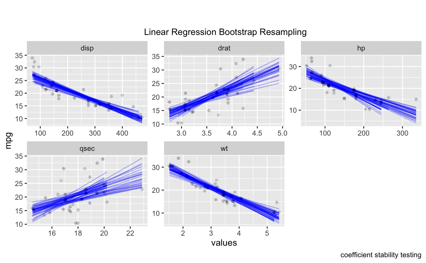
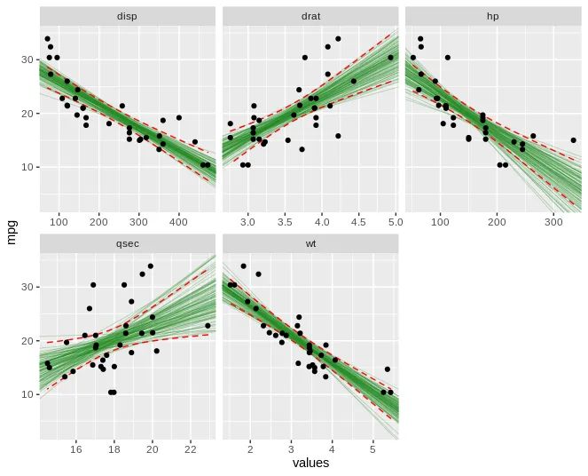
ggplot(boot_aug_total_2, aes(values, mpg)) +
geom_line(aes(y = .fitted, group = id), alpha = .3, col = "blue") +
geom_point(alpha = 0.005) +
labs(title="", subtitle = " \n Linear Regression Bootstrap Resampling") +
theme(plot.title = element_text(hjust = 0.5, face = "bold")) +
theme(plot.subtitle = element_text(hjust = 0.5)) +
labs(caption = "coefficient stability testing") +
facet_wrap(~factor, scales = 'free')
对比


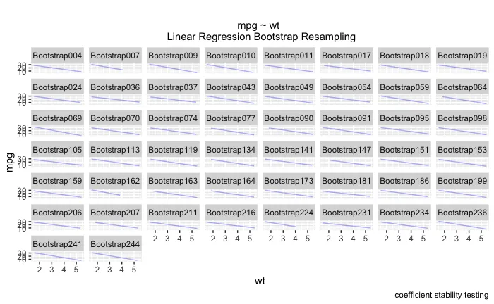


facet_wrap(),还是类似ggarrange()的方法也可以?后者更简单易行,但集成度更低、更不紧凑。如果你愿意,我可以发布一个使用非 facet 方式的示例作为答案。 - Skaqqs