使用Python和Mayavi创建3D流线图

Question

最近，Tom Flannaghan和Tony Yu将streamplot纳入matplotlib中，因此使用python和matplotlib生成2D流图非常容易。

尽管可以使用matplotlib生成某些类型的3D图，但目前不支持3D流图。然而，Python绘图程序mayavi（提供基于vtk的绘图的Python接口）可以使用其flow()函数生成3D流图。

我创建了一个简单的Python模块来在2D和3D中流绘制数据，其中3D数据集中没有Z坡度（所有dZ = 0），以展示我在mayavi与matplotlib上面对匹配xy平面数据绘图挑战的情况。以下是有注释的代码和生成的图形：

import numpy, matplotlib, mayavi, matplotlib.pyplot, mayavi.mlab
#for now, let's produce artificial streamline data sets for 2D & 3D cases where x and y change by +1 at each point, while Z changes by 0 at each point:

#2D data first:
x = numpy.ones((10,10))
y = numpy.ones((10,10))
#and a corresponding meshgrid:
Y,X = numpy.mgrid[-10:10:10j,-10:10:10j]

#now 3D data with Z = 0 (i.e., I want to be able to produce a matching streamplot plane in mayavi, which is normally used for 3D):
xx = numpy.ones((10,10,10))
yy = numpy.ones((10,10,10))
zz = numpy.zeros((10,10,10))
#and a corresponding meshgrid:
ZZ,YY,XX = numpy.mgrid[-10:10:10j,-10:10:10j,-10:10:10j]

#plot the 2D streamplot data with matplotlib:
fig = matplotlib.pyplot.figure()
ax = fig.add_subplot(111,aspect='equal')
speed = numpy.sqrt(x*x + y*y)
ax.streamplot(X, Y, x, y, color=x, linewidth=2, cmap=matplotlib.pyplot.cm.autumn,arrowsize=3)
fig.savefig('test_streamplot_2D.png',dpi=300)

#there's no streamplot 3D available in matplotlib, so try to see how mayavi behaves with a similar 3D data set:
fig = mayavi.mlab.figure(bgcolor=(1.0,1.0,1.0),size=(800,800),fgcolor=(0, 0, 0))
st = mayavi.mlab.flow(XX,YY,ZZ,xx,yy,zz,line_width=4,seedtype='sphere',integration_direction='forward') #sphere is the default seed type
mayavi.mlab.axes(extent = [-10.0,10.0,-10.0,10.0,-1.0,1.0]) #set plot bounds
fig.scene.z_plus_view() #adjust the view for a perspective along z (xy plane flat)
mayavi.mlab.savefig('test_streamplot_3D_attempt_1.png')

#now start to modify the mayavi code to see if I can 'seed in' more streamlines (default only produces a single short streamline, albeit of the correct slope)
#attempt 2 uses a line seed / widget over the specified bounds (points 1 and 2):
fig = mayavi.mlab.figure(bgcolor=(1.0,1.0,1.0),size=(800,800),fgcolor=(0, 0, 0))
st = mayavi.mlab.flow(XX,YY,ZZ,xx,yy,zz,line_width=4,seedtype='line',integration_direction='forward') #line instead of sphere
st.seed.widget.point1 = [0,-10,0]
st.seed.widget.point2 = [0,10,0] #so seed line should go up along y axis
st.seed.widget.resolution = 25 #seems to be the number of seeds points along the seed line
mayavi.mlab.axes(extent = [-10.0,10.0,-10.0,10.0,-1.0,1.0]) #set plot bounds
fig.scene.z_plus_view() #adjust the view for a perspective along z (xy plane flat)
mayavi.mlab.savefig('test_streamplot_3D_attempt_2.png')

#attempt 3 will try to seed a diagonal line across the plot to produce streamlines that cover the full plot:
#would need to use 'both' for integration_direction if I could get the diagonal seed line to work
fig = mayavi.mlab.figure(bgcolor=(1.0,1.0,1.0),size=(800,800),fgcolor=(0, 0, 0)) 
st = mayavi.mlab.flow(XX,YY,ZZ,xx,yy,zz,line_width=4,seedtype='line',integration_direction='forward') 
st.seed.widget.point1 = [-10,10,0] #start seed line at top left corner of plot
st.seed.widget.point2 = [10,-10,0] #end seed line at bottom right corner of plot 
#this fails to produce a diagonal seed line though
st.seed.widget.resolution = 25 #seems to be the number of seeds points along the seed line
mayavi.mlab.axes(extent = [-10.0,10.0,-10.0,10.0,-1.0,1.0]) #set plot bounds
fig.scene.z_plus_view() #adjust the view for a perspective along z (xy plane flat)
mayavi.mlab.savefig('test_streamplot_3D_attempt_3.png')

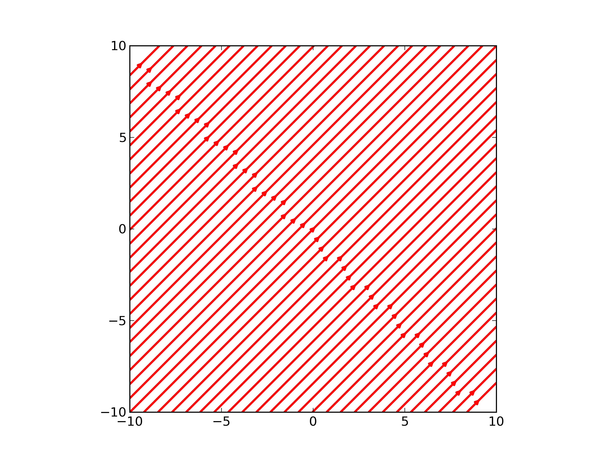
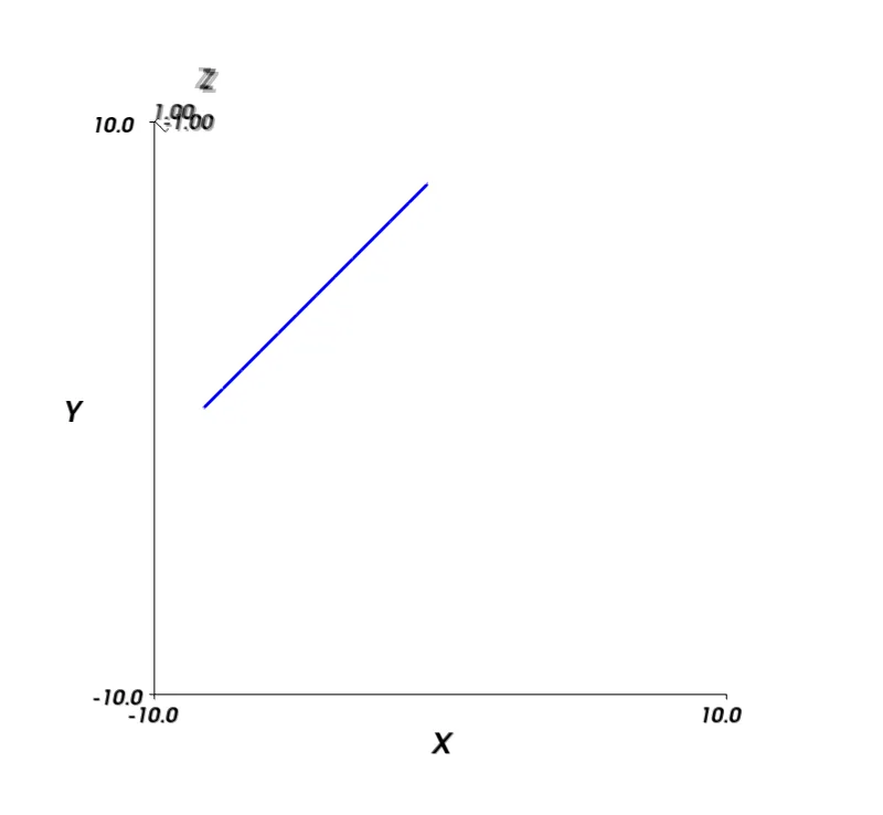
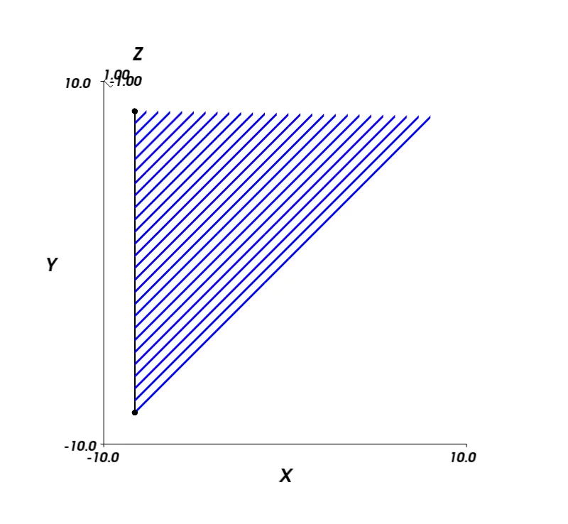
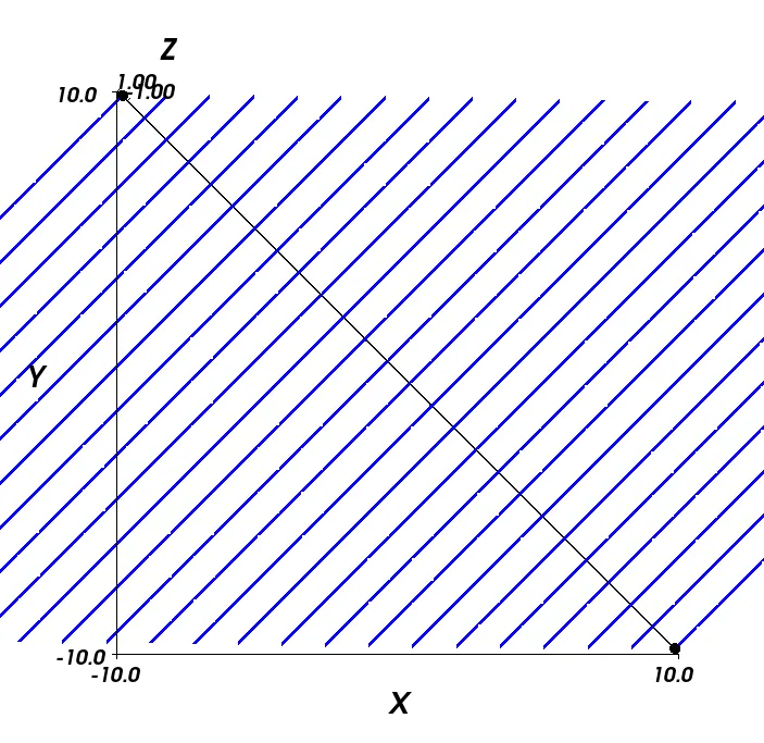
2D matplotlib结果（请注意，斜率为1的流线与填充有单位值的dx和dy数组相匹配）： 3D mayavi结果（尝试1; 请注意，单个流线的斜率是正确的，但流线的长度和数量显然与2D matplotlib示例不同）： 3D mayavi结果（尝试2; 请注意，我使用具有足够高分辨率的线种子产生了更多适当斜率的流线，但是请注意，在代码中指定的黑色种子线的起始和结束x坐标与绘图不匹配） 最后，尝试＃3（令人困惑地）产生与＃2完全相同的情节，尽管指定了不同的种子/小部件点。因此，问题是：如何更好地控制我的种子线的位置使其成为对角线？更广泛地说，我想能够输入任意阵列的种子点以解决更一般的流图3D（非平面）问题，但是解决前者特定情况的线条应该让我开始。

在解决这个问题时，我找到了一些其他有用的资源，但它们并没有完全解决我的问题：

1. matplotlib的streamplot共同作者Tom Flannaghan在博客文章中讨论了这个主题
2. 一个示例，其中使用自定义种子数组与mayavi Streamline子类（其又被flow（）使用），但遗憾的是缺乏足够的实现细节无法复现。
3. 使用mayavi生成二维磁力线流图的示例，包括注释源代码。
4. 带有三维源代码的类似示例，但仍然无法解决我的绘图问题：
5. mayavi标准文档提供的flow() 绘图结果示例代码（流线后面可见球形种子小部件）。

- treddy

Answer 1

看起来问题是流线种子小部件的clamp_to_bounds属性的默认值被设置为True。您必须将其设置为False才能实际移动该小部件。

st.seed.widget.clamp_to_bounds = False

在将此代码添加后，最终结果如下所示： 您可能之前就熟悉了从Mayavi中探索的方法，但为了避免解释过多，我还是会提到：我通常通过启用pylab来运行IPython脚本来找到Mayavi中这种模糊属性的选项。在Ubuntu上，终端命令如下：

ipython --pylab=qt

在启动IPython后，我使用%run魔法命令运行脚本：

%run streamlines.py

制作完图表后，现在我可以通过点击Mayavi图标来访问Mayavi窗口并查看Mayavi管道的内部情况:

在管道中，您会找到Streamline对象，如果单击它，然后选择Seed，您将找到"Clamp to bounds"复选框。(抱歉截图中颜色混乱 - 最近Mayavi出现了一些奇怪的使用暗色主题的原因...)

要查看这实际上是做什么的，您可以点击记录按钮打开一个窗口，显示您更改设置的代码等效项：

在那里，您可以看到clamp_to_bounds属性，并能够将其添加到您的脚本中。

祝您在流线方面好运！

- dragly