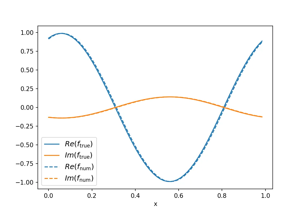
在Python中使用隐式欧拉法解决PDE - 输出不正确

Question

在Python中使用隐式欧拉法解决PDE - 输出不正确

14

我会尝试解释正在发生的事情和我的问题。

这有点数学化，SO不支持LaTeX，所以不幸的是我不得不使用图片。希望这没关系。

我不知道为什么它是倒置的，很抱歉。无论如何，这是一个线性系统Ax = b，我们知道A和b，因此我们可以找到x，这是我们在下一个时间步长的近似值。我们继续这样做直到t_final时间。这是代码。

import numpy as np

tau = 2 * np.pi
tau2 = tau * tau
i = complex(0,1)

def solution_f(t, x):
    return 0.5 * (np.exp(-tau * i * x) * np.exp((2 - tau2) * i * t) + np.exp(tau * i * x) * np.exp((tau2 + 4) * i * t))

def solution_g(t, x):
    return 0.5 * (np.exp(-tau * i * x) * np.exp((2 - tau2) * i * t) - np.exp(tau * i * x) * np.exp((tau2 + 4) * i * t))

for l in range(2, 12):
    N = 2 ** l #number of grid points
    dx = 1.0 / N #space between grid points
    dx2 = dx * dx
    dt = dx #time step
    t_final = 1
    approximate_f = np.zeros((N, 1), dtype = np.complex)
    approximate_g = np.zeros((N, 1), dtype = np.complex)

    #Insert initial conditions
    for k in range(N):
        approximate_f[k, 0] = np.cos(tau * k * dx)
        approximate_g[k, 0] = -i * np.sin(tau * k * dx)

    #Create coefficient matrix
    A = np.zeros((2 * N, 2 * N), dtype = np.complex)

    #First row is special
    A[0, 0] = 1 -3*i*dt
    A[0, N] = ((2 * dt / dx2) + dt) * i
    A[0, N + 1] = (-dt / dx2) * i
    A[0, -1] = (-dt / dx2) * i

    #Last row is special
    A[N - 1, N - 1] = 1 - (3 * dt) * i
    A[N - 1, N] = (-dt / dx2) * i
    A[N - 1, -2] = (-dt / dx2) * i
    A[N - 1, -1] = ((2 * dt / dx2) + dt) * i

    #middle
    for k in range(1, N - 1):
        A[k, k] = 1 - (3 * dt) * i
        A[k, k + N - 1] = (-dt / dx2) * i
        A[k, k + N] = ((2 * dt / dx2) + dt) * i
        A[k, k + N + 1] = (-dt / dx2) * i

    #Bottom half
    A[N :, :N] = A[:N, N:]
    A[N:, N:] = A[:N, :N]

    Ainv = np.linalg.inv(A)

    #Advance through time
    time = 0
    while time < t_final:
        b = np.concatenate((approximate_f, approximate_g), axis = 0)
        x = np.dot(Ainv, b) #Solve Ax = b
        approximate_f = x[:N]
        approximate_g = x[N:]
        time += dt
    approximate_solution = np.concatenate((approximate_f, approximate_g), axis=0)

    #Calculate the actual solution
    actual_f = np.zeros((N, 1), dtype = np.complex)
    actual_g = np.zeros((N, 1), dtype = np.complex)
    for k in range(N):
        actual_f[k, 0] = solution_f(t_final, k * dx)
        actual_g[k, 0] = solution_g(t_final, k * dx)
    actual_solution = np.concatenate((actual_f, actual_g), axis = 0)

    print(np.sqrt(dx) * np.linalg.norm(actual_solution - approximate_solution))

它不起作用。至少在开始时，它不应该这么慢。它应该是无条件稳定的，并收敛到正确的答案。

这里出了什么问题？

- Oria Gruber

2个回答

-1

我不打算逐个计算你的数学问题，但我会给出一个建议。

直接计算f_xx和g_xx似乎是一个可能存在数值不稳定性的好选择。直觉上，一阶方法应该会在项中产生二阶误差。通过该公式后，二阶误差在二阶导数中变成常数阶的误差。此外，当步长变小时，你会发现二次公式会将即使是微小的舍入误差转化为令人惊讶的大误差。

相反地，我建议你首先将其转化为一个由4个函数组成的一阶系统，即f、f_x、g和g_x。然后在该系统上采用向后欧拉法进行计算。凭直觉来说，采用这种方法，一阶方法会产生二阶误差，然后通过一个公式产生它们的一阶误差。现在你从一开始就收敛了，并且对舍入误差的传播也不敏感。

- btilly

网页内容由stack overflow 提供, 点击上面的

可以查看英文原文，
原文链接

- Doe a · Accepted Answer

L2范数可以作为测试收敛性的有用指标，但在调试时并不理想，因为它不能解释问题所在。虽然您的解决方案应该是无条件稳定的，但向后欧拉不一定会收敛到正确的答案。就像向前欧拉一样，向后欧拉也以不稳定（反耗散）而闻名。绘制您的解决方案可以证实这一点。数值解收敛于零。对于下一个级别的近似，Crank-Nicolson是一个合理的选择。以下代码包含了更一般的theta方法，以便您可以调整隐含性。theta = 0.5表示CN，theta = 1表示BE，theta = 0表示FE。我进行了一些微调：

我选择了一个更适当的时间步长dt =（dx ** 2）/ 2，而不是dt = dx。后者使用CN不会收敛到正确的解。
这是一个小细节，但由于t_final不能保证是dt的倍数，您没有在同一时间步上比较解。
关于您关于速度慢的评论：随着空间分辨率的增加，您的时间分辨率也需要增加。即使在dt = dx的情况下，你也必须执行（1024x1024）* 1024矩阵乘法1024次。我并没有发现这在我的机器上需要太长时间。我删除了一些不必要的连接以加快速度，但将时间步长更改为dt =（dx ** 2）/ 2将使事情变慢，不幸的是。如果您担心速度，请尝试使用Numba编译。

总之，我在CN的一致性方面没有取得很大的成功。我必须设置N = 2 ^ 6才能在t_final = 1时获得任何东西。增加t_final会使情况变得更糟，减少t_final会使情况变得更好。根据您的需求，您可以考虑实施TR-BDF2或其他线性多步方法来改善这种情况。

带有绘图的代码如下：

import numpy as np
import matplotlib.pyplot as plt

tau = 2 * np.pi
tau2 = tau * tau
i = complex(0,1)

def solution_f(t, x):
    return 0.5 * (np.exp(-tau * i * x) * np.exp((2 - tau2) * i * t) + np.exp(tau * i * x) * np.exp((tau2 + 4) * i * t))

def solution_g(t, x):
    return 0.5 * (np.exp(-tau * i * x) * np.exp((2 - tau2) * i * t) - np.exp(tau * i * x) * 
np.exp((tau2 + 4) * i * t))

l=6
N = 2 ** l 
dx = 1.0 / N 
dx2 = dx * dx
dt = dx2/2
t_final = 1.
x_arr = np.arange(0,1,dx)

approximate_f = np.cos(tau*x_arr)
approximate_g = -i*np.sin(tau*x_arr)

H = np.zeros([2*N,2*N], dtype=np.complex)
for k in range(N):
    H[k,k] = -3*i*dt
    H[k,k+N] = (2/dx2+1)*i*dt    
    if k==0:
        H[k,N+1] = -i/dx2*dt
        H[k,-1] = -i/dx2*dt     
    elif k==N-1:
        H[N-1,N] = -i/dx2*dt
        H[N-1,-2] = -i/dx2*dt    
    else:
        H[k,k+N-1] = -i/dx2*dt
        H[k,k+N+1] = -i/dx2*dt
### Bottom half
H[N :, :N] = H[:N, N:]
H[N:, N:] = H[:N, :N]

### Theta method. 0.5 -> Crank Nicolson
theta=0.5
A = np.eye(2*N)+H*theta
B = np.eye(2*N)-H*(1-theta)

### Precompute for faster computations
mat = np.linalg.inv(A)@B

t = 0
b = np.concatenate((approximate_f, approximate_g))
while t < t_final:
    t += dt
    b = mat@b

approximate_f = b[:N]
approximate_g = b[N:]
approximate_solution = np.concatenate((approximate_f, approximate_g))

#Calculate the actual solution
actual_f = solution_f(t,np.arange(0,1,dx))
actual_g = solution_g(t,np.arange(0,1,dx))
actual_solution = np.concatenate((actual_f, actual_g))

plt.figure(figsize=(7,5))
plt.plot(x_arr,actual_f.real,c="C0",label=r"$Re(f_\mathrm{true})$")
plt.plot(x_arr,actual_f.imag,c="C1",label=r"$Im(f_\mathrm{true})$")
plt.plot(x_arr,approximate_f.real,c="C0",ls="--",label=r"$Re(f_\mathrm{num})$")
plt.plot(x_arr,approximate_f.imag,c="C1",ls="--",label=r"$Im(f_\mathrm{num})$")
plt.legend(loc=3,fontsize=12)
plt.xlabel("x")

plt.savefig("num_approx.png",dpi=150)