我如何在图像上应用这些 Gabor 滤波小波?
close all;
clear all;
clc;
% Parameter Setting
R = 128;
C = 128;
Kmax = pi / 2;
f = sqrt( 2 );
Delt = 2 * pi;
Delt2 = Delt * Delt;
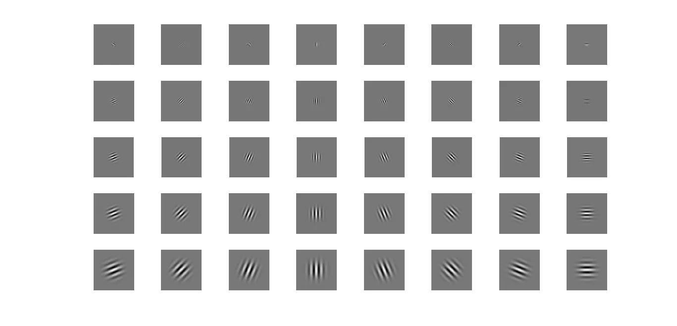
% Show the Gabor Wavelets
for v = 0 : 4
for u = 1 : 8
GW = GaborWavelet ( R, C, Kmax, f, u, v, Delt2 ); % Create the Gabor wavelets
figure( 2 );
subplot( 5, 8, v * 8 + u ),imshow ( real( GW ) ,[]); % Show the real part of Gabor wavelets
end
figure ( 3 );
subplot( 1, 5, v + 1 ),imshow ( abs( GW ),[]); % Show the magnitude of Gabor wavelets
end
function GW = GaborWavelet (R, C, Kmax, f, u, v, Delt2)
k = ( Kmax / ( f ^ v ) ) * exp( 1i * u * pi / 8 );% Wave Vector
kn2 = ( abs( k ) ) ^ 2;
GW = zeros ( R , C );
for m = -R/2 + 1 : R/2
for n = -C/2 + 1 : C/2
GW(m+R/2,n+C/2) = ( kn2 / Delt2 ) * exp( -0.5 * kn2 * ( m ^ 2 + n ^ 2 ) / Delt2) * ( exp( 1i * ( real( k ) * m + imag ( k ) * n ) ) - exp ( -0.5 * Delt2 ) );
end
end
编辑:这是我的图片尺寸
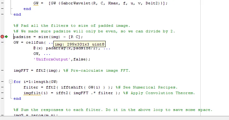
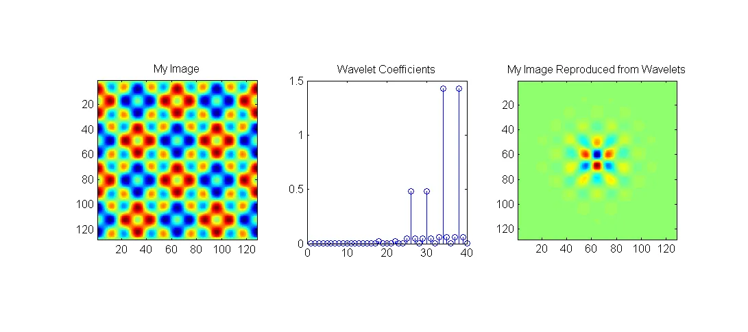 修改如下:
修改如下: