我想知道是否可能以类似于matlab的Profiler的方式从R-Code中获取配置文件。也就是说,了解哪些行号特别慢。
到目前为止,我所取得的成果并不令人满意。我使用Rprof制作了一个配置文件。使用summaryRprof,我得到了以下内容:
所以我尝试了Hadley Wickham的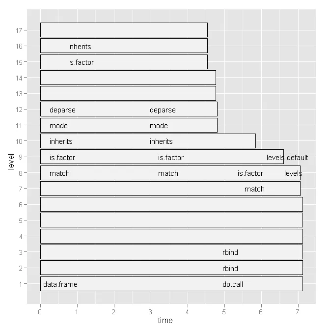 有没有更方便的方法可以查看哪些行号和特定函数调用很慢?
或者,有没有一些文献应该参考?
有没有更方便的方法可以查看哪些行号和特定函数调用很慢?
或者,有没有一些文献应该参考?
任何提示都会受到赞赏。
编辑1: 根据Hadley的评论,我将在下面粘贴我的脚本代码和绘图的基本版本。但请注意,我的问题与此特定脚本无关。这只是我最近编写的一个随机脚本。我正在寻找一般的方法来查找瓶颈并加速R代码。
数据(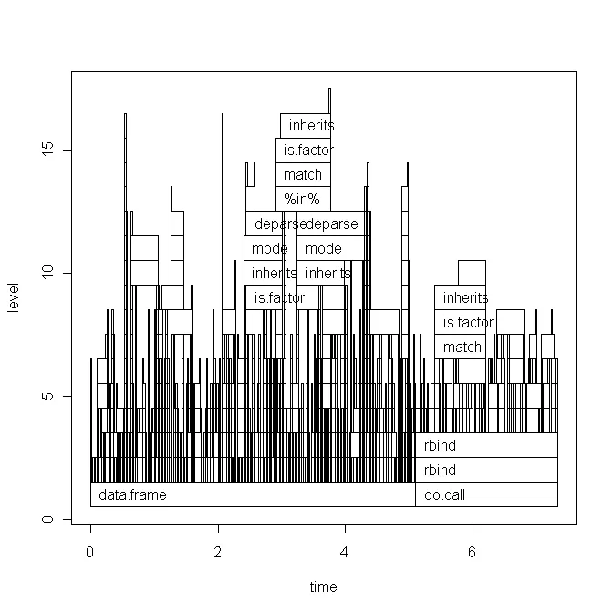 今天运行脚本还稍微改变了ggplot2图表(基本上只有标签),请看这里。
到目前为止,我所取得的成果并不令人满意。我使用Rprof制作了一个配置文件。使用summaryRprof,我得到了以下内容:
$by.self
                  self.time self.pct total.time total.pct
[.data.frame               0.72     10.1       1.84      25.8
inherits                   0.50      7.0       1.10      15.4
data.frame                 0.48      6.7       4.86      68.3
unique.default             0.44      6.2       0.48       6.7
deparse                    0.36      5.1       1.18      16.6
rbind                      0.30      4.2       2.22      31.2
match                      0.28      3.9       1.38      19.4
[<-.factor                 0.28      3.9       0.56       7.9
levels                     0.26      3.7       0.34       4.8
NextMethod                 0.22      3.1       0.82      11.5
...
并且。
$by.total
                      total.time total.pct self.time self.pct
data.frame                  4.86      68.3      0.48      6.7
rbind                       2.22      31.2      0.30      4.2
do.call                     2.22      31.2      0.00      0.0
[                           1.98      27.8      0.16      2.2
[.data.frame                1.84      25.8      0.72     10.1
match                       1.38      19.4      0.28      3.9
%in%                        1.26      17.7      0.14      2.0
is.factor                   1.20      16.9      0.10      1.4
deparse                     1.18      16.6      0.36      5.1
...
坦白地说,从这个输出中,我不知道我的瓶颈在哪里,因为(a)我经常使用data.frame,(b)我从未使用例如deparse。此外,[是什么?所以我尝试了Hadley Wickham的
profr,但是考虑到以下图表,它并没有更有用:
有没有更方便的方法可以查看哪些行号和特定函数调用很慢?
或者,有没有一些文献应该参考?任何提示都会受到赞赏。
编辑1: 根据Hadley的评论,我将在下面粘贴我的脚本代码和绘图的基本版本。但请注意,我的问题与此特定脚本无关。这只是我最近编写的一个随机脚本。我正在寻找一般的方法来查找瓶颈并加速R代码。
数据(
x)看起来像这样:
type      word    response    N   Classification  classN
Abstract  ANGER   bitter      1   3a              3a
Abstract  ANGER   control     1   1a              1a
Abstract  ANGER   father      1   3a              3a
Abstract  ANGER   flushed     1   3a              3a
Abstract  ANGER   fury        1   1c              1c
Abstract  ANGER   hat         1   3a              3a
Abstract  ANGER   help        1   3a              3a
Abstract  ANGER   mad         13  3a              3a
Abstract  ANGER   management  2   1a              1a
... until row 1700
脚本(附有简短的解释)如下所示:
Rprof("profile1.out")

# A new dataset is produced with each line of x contained x$N times
y <- vector('list',length(x[,1]))
for (i in 1:length(x[,1])) {
  y[[i]] <- data.frame(rep(x[i,1],x[i,"N"]),rep(x[i,2],x[i,"N"]),rep(x[i,3],x[i,"N"]),rep(x[i,4],x[i,"N"]),rep(x[i,5],x[i,"N"]),rep(x[i,6],x[i,"N"]))
}
all <- do.call('rbind',y)
colnames(all) <- colnames(x)

# create a dataframe out of a word x class table
table_all <- table(all$word,all$classN)
dataf.all <- as.data.frame(table_all[,1:length(table_all[1,])])
dataf.all$words <- as.factor(rownames(dataf.all))
dataf.all$type <- "no"
# get type of the word.
words <- levels(dataf.all$words)
for (i in 1:length(words)) {
  dataf.all$type[i] <- as.character(all[pmatch(words[i],all$word),"type"])
}
dataf.all$type <- as.factor(dataf.all$type)
dataf.all$typeN <- as.numeric(dataf.all$type)

# aggregate response categories
dataf.all$c1 <- apply(dataf.all[,c("1a","1b","1c","1d","1e","1f")],1,sum)
dataf.all$c2 <- apply(dataf.all[,c("2a","2b","2c")],1,sum)
dataf.all$c3 <- apply(dataf.all[,c("3a","3b")],1,sum)

Rprof(NULL)

library(profr)
ggplot.profr(parse_rprof("profile1.out"))
最终数据如下:
1a    1b  1c  1d  1e  1f  2a  2b  2c  3a  3b  pa  words   type    typeN   c1  c2  c3  pa
3 0   8   0   0   0   0   0   0   24  0   0   ANGER   Abstract    1   11  0   24  0
6 0   4   0   1   0   0   11  0   13  0   0   ANXIETY Abstract    1   11  11  13  0
2 11  1   0   0   0   0   4   0   17  0   0   ATTITUDE    Abstract    1   14  4   17  0
9 18  0   0   0   0   0   0   0   0   8   0   BARREL  Concrete    2   27  0   8   0
0 1   18  0   0   0   0   4   0   12  0   0   BELIEF  Abstract    1   19  4   12  0
基本的图形绘制:
今天运行脚本还稍微改变了ggplot2图表(基本上只有标签),请看这里。
plot而不是ggplot吗?同时看到你的原始代码会很有用。 - hadley