我需要绘制一个柱状图来显示计数,同时又要绘制一条折线图来显示比率,两者需要在同一张图表中呈现。我可以分别绘制它们,但当我将它们放在一起时,第一层(即 geom_bar)的比例尺被第二层(即 geom_line)遮盖。
我能否将 geom_line 的坐标轴移到右侧?
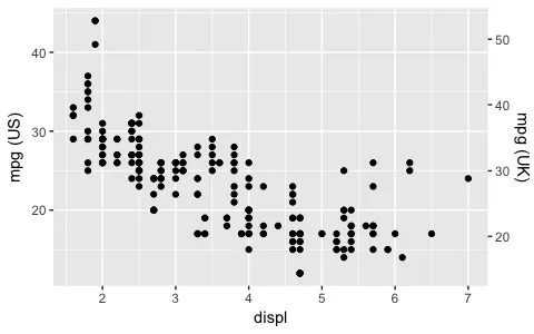
从ggplot2 2.2.0开始,您可以像这样添加第二个轴(摘自ggplot2 2.2.0公告):
ggplot(mpg, aes(displ, hwy)) +
  geom_point() +
  scale_y_continuous(
    "mpg (US)",
    <b>sec.axis = sec_axis(~ . * 1.20, name = "mpg (UK)")</b>
  )
在ggplot2中,不可能实现这一点,因为我相信具有独立y轴刻度(而不是互相变换的y轴刻度)的图表从根本上存在缺陷。以下是一些问题:
它们不可逆:给定图形空间中的一个点,无法将其唯一地映射回数据空间中的一个点。
与其他选项相比,它们相对难以正确阅读。请参见Petra Isenberg、Anastasia Bezerianos、Pierre Dragicevic和Jean-Daniel Fekete的文章《双刻度数据图表研究》了解详情。
它们很容易被操纵误导:没有唯一的方法来指定坐标轴的相对比例,使它们容易受到操纵。Junkcharts博客上的两个例子:一个,两个
它们是任意的:为什么只有2个刻度,而不是3、4或10个?
你可能还想阅读Stephen Few的详细讨论:图表中的双刻度轴——它们真的是最好的解决方案吗?。
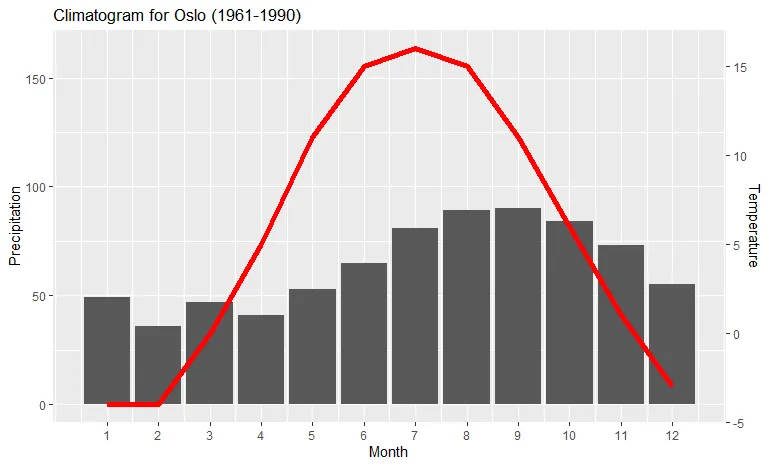
存在一些通用的双Y轴使用场景,例如展示月平均气温和降水量的气象图。这里提供了一个简单的解决方案,是建立在 Megatron 的基础上并允许您设置变量的下限而不一定是零:
示例数据:
climate <- tibble(
  Month = 1:12,
  Temp = c(-4,-4,0,5,11,15,16,15,11,6,1,-3),
  Precip = c(49,36,47,41,53,65,81,89,90,84,73,55)
  )
将以下两个值设置为接近数据极限的值(您可以尝试调整这些值以调整图表位置;轴仍将正确):
将以下两个值设置为靠近数据极限的值(您可以根据需要进行微调,来调整图表位置;坐标轴将保持正确):
ylim.prim <- c(0, 180)   # in this example, precipitation
ylim.sec <- c(-4, 18)    # in this example, temperature
b <- diff(ylim.prim)/diff(ylim.sec)
a <- ylim.prim[1] - b*ylim.sec[1]) # there was a bug here

ggplot(climate, aes(Month, Precip)) +
  geom_col() +
  geom_line(aes(y = a + Temp*b), color = "red") +
  scale_y_continuous("Precipitation", sec.axis = sec_axis(~ (. - a)/b, name = "Temperature")) +
  scale_x_continuous("Month", breaks = 1:12) +
  ggtitle("Climatogram for Oslo (1961-1990)")
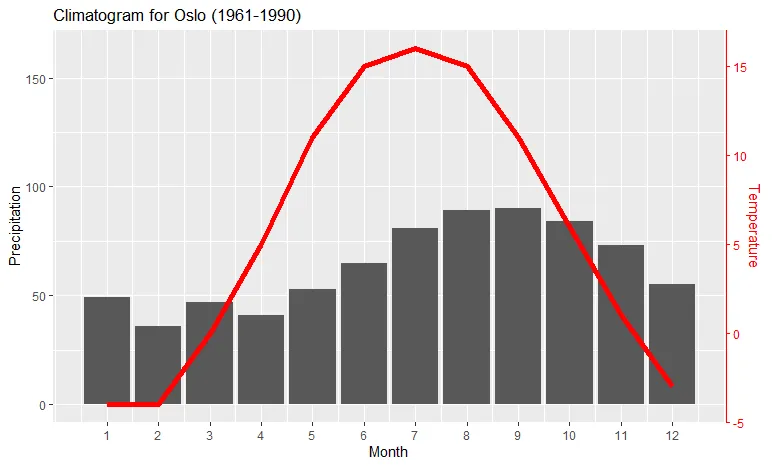
如果您想确保红色线对应右侧的y轴,您可以向代码添加一个theme语句:
ggplot(climate, aes(Month, Precip)) +
  geom_col() +
  geom_line(aes(y = a + Temp*b), color = "red") +
  scale_y_continuous("Precipitation", sec.axis = sec_axis(~ (. - a)/b, name = "Temperature")) +
  scale_x_continuous("Month", breaks = 1:12) +
  theme(axis.line.y.right = element_line(color = "red"),
        axis.ticks.y.right = element_line(color = "red"),
        axis.text.y.right = element_text(color = "red"),
        axis.title.y.right = element_text(color = "red")
        ) +
  ggtitle("Climatogram for Oslo (1961-1990)")
将右侧轴线的颜色更改为红色:
ylim.prim 和 ylim.sec 的值处中断。 - Eric Krantzylim.prim[1] - b*ylim.sec[1]) 后面写了 "there was a bug here",我认为最后不应该有一个 )。 - undefined您可以创建一个缩放因子,该因子应用于第二个geom和右y轴。这是从Sebastian的解决方案中推导出来的。
library(ggplot2)

scaleFactor <- max(mtcars$cyl) / max(mtcars$hp)

ggplot(mtcars, aes(x=disp)) +
  geom_smooth(aes(y=cyl), method="loess", col="blue") +
  geom_smooth(aes(y=hp * scaleFactor), method="loess", col="red") +
  scale_y_continuous(name="cyl", sec.axis=sec_axis(~./scaleFactor, name="hp")) +
  theme(
    axis.title.y.left=element_text(color="blue"),
    axis.text.y.left=element_text(color="blue"),
    axis.title.y.right=element_text(color="red"),
    axis.text.y.right=element_text(color="red")
  )
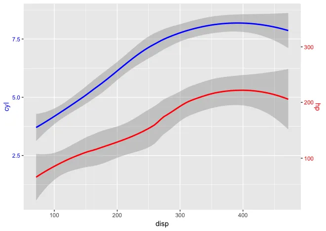
注意:使用 ggplot2 v3.0.0
双手赞成 - SilSur根据以上回答,并进行一些微调后(不管值不值得),以下是通过 sec_axis 实现两个比例尺的方法:
假设有一个简单的(纯虚构的)数据集 dt: 在五天内,它跟踪了干扰次数与生产率之间的关系:
        when numinter prod
1 2018-03-20        1 0.95
2 2018-03-21        5 0.50
3 2018-03-23        4 0.70
4 2018-03-24        3 0.75
5 2018-03-25        4 0.60
(两列数据的范围相差约为5倍)。
以下代码将绘制这两个系列,以便它们占用整个y轴:
ggplot() +
  geom_bar(mapping = aes(x = dt$when, y = dt$numinter), stat = "identity", fill = "grey") +
  geom_line(mapping = aes(x = dt$when, y = dt$prod*5), size = 2, color = "blue") +
  scale_x_date(name = "Day", labels = NULL) +
  scale_y_continuous(name = "Interruptions/day",
    sec.axis = sec_axis(~./5, name = "Productivity % of best",
      labels = function(b) { paste0(round(b * 100, 0), "%")})) +
  theme(
      axis.title.y = element_text(color = "grey"),
      axis.title.y.right = element_text(color = "blue"))
这是上面代码加一些调色后的结果:
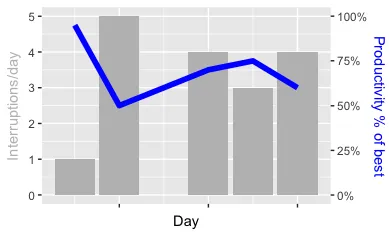
除了使用sec_axis来指定y轴比例以外,重点是在指定数据系列时将第二个数据系列的每个值乘以5。为了正确设置sec_axis中的标签,需要除以5(并进行格式化)。因此,以上代码中一个至关重要的部分是在geom_line中的*5和在sec_axis中的~./5(一个公式将当前值.除以5)。
相比之下(我不想评判这两种方法),这就是堆叠在一起的两个图表的样子:
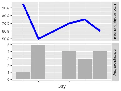
你可以自己判断哪一个更好地传达了信息(“不要打扰工作中的人!”)。我想这是一个公平的决定方式。
两张图片的完整代码(实际上不会比以上内容多太多,只是完整而已,可以直接运行)在这里:https://gist.github.com/sebastianrothbucher/de847063f32fdff02c83b75f59c36a7d 更详细的解释在这里:https://sebastianrothbucher.github.io/datascience/r/visualization/ggplot/2018/03/24/two-scales-ggplot-r.html
scale_y_continuous的labels参数的输入,那就太好了。 - James Hirschornlibrary(ggplot2)
library(scales)
# Function factory for secondary axis transforms
train_sec <- function(primary, secondary, na.rm = TRUE) {
# Thanks Henry Holm for including the na.rm argument!
from <- range(secondary, na.rm = na.rm)
to <- range(primary, na.rm = na.rm)
# Forward transform for the data
forward <- function(x) {
rescale(x, from = from, to = to)
}
# Reverse transform for the secondary axis
reverse <- function(x) {
rescale(x, from = to, to = from)
}
list(fwd = forward, rev = reverse)
}
这似乎相当复杂,但是制作函数工厂可以使所有其他操作变得更加容易。现在,在我们制作图表之前,我们将通过向工厂展示主要和次要数据来生成相关函数。我们将使用经济数据集,该数据集的unemploy和psavert列具有非常不同的范围。
sec <- with(economics, train_sec(unemploy, psavert))
y = sec$fwd(psavert)将辅助数据重新调整到主轴,并将~ sec$rev(.)指定为辅助轴的转换参数。这样,我们就可以得到一个图表,其中主轴和辅助轴的范围在图表上占据相同的空间。ggplot(economics, aes(date)) +
geom_line(aes(y = unemploy), colour = "blue") +
geom_line(aes(y = sec$fwd(psavert)), colour = "red") +
scale_y_continuous(sec.axis = sec_axis(~sec$rev(.), name = "psavert"))

工厂比这个稍微灵活一些,因为如果你只想重新缩放最大值,你可以传入下限为0的数据。
# Rescaling the maximum
sec <- with(economics, train_sec(c(0, max(unemploy)),
c(0, max(psavert))))
ggplot(economics, aes(date)) +
  geom_line(aes(y = unemploy), colour = "blue") +
  geom_line(aes(y = sec$fwd(psavert)), colour = "red") +
  scale_y_continuous(sec.axis = sec_axis(~sec$rev(.), name = "psavert"))

该示例创建于2021年02月05日,使用reprex package(v0.3.0)。
我承认在此示例中差异并不是非常明显,但如果您仔细观察,就会发现最大值相同,而红线比蓝线更低。
编辑:
此方法现已在ggh4x软件包的help_secondary()函数中进行捕获和扩展。免责声明:我是ggh4x的作者。
  df <- data.frame(item=LETTERS[1:n],  y1=c(-0.8684, 4.2242, -0.3181, 0.5797, -0.4875), y2=c(-5.719, 205.184, 4.781, 41.952, 9.911 )) # made up!

> df
  item      y1         y2
1    A -0.8684 -19.154567
2    B  4.2242 219.092499
3    C -0.3181  18.849686
4    D  0.5797  46.945161
5    E -0.4875  -4.721973
ggplot(data=df, aes(label=item)) +
  theme_bw() +
  geom_segment(aes(x='G1', xend='G2', y=y1, yend=y2), color='grey')+
  geom_text(aes(x='G1', y=y1), color='blue') +
  geom_text(aes(x='G2', y=y2), color='red') +
  theme(legend.position='none', panel.grid=element_blank())
它不能很好地对齐,因为较小比例的y1被较大比例的y2明显压缩。
在这里应对挑战的诀窍是技术上绘制两个数据集针对第一个比例y1,但报告第二个针对具有显示原始比例y2标签的次要轴。
因此,我们构建了第一个帮助函数CalcFudgeAxis,该函数计算并收集要显示的新轴的特征。该函数可以根据任何人的喜好进行修改(此函数仅将y2映射到y1的范围内)。
CalcFudgeAxis = function( y1, y2=y1) {
  Cast2To1 = function(x) ((ylim1[2]-ylim1[1])/(ylim2[2]-ylim2[1])*x) # x gets mapped to range of ylim2
  ylim1 <- c(min(y1),max(y1))
  ylim2 <- c(min(y2),max(y2))
  yf <- Cast2To1(y2)
  labelsyf <- pretty(y2)
  return(list(
    yf=yf,
    labels=labelsyf,
    breaks=Cast2To1(labelsyf)
  ))
}
什么会产生一些:
> FudgeAxis <- CalcFudgeAxis( df$y1, df$y2 )

> FudgeAxis
$yf
[1] -0.4094344  4.6831656  0.4029175  1.0034664 -0.1009335

$labels
[1] -50   0  50 100 150 200 250

$breaks
[1] -1.068764  0.000000  1.068764  2.137529  3.206293  4.275058  5.343822


> cbind(df, FudgeAxis$yf)
  item      y1         y2 FudgeAxis$yf
1    A -0.8684 -19.154567   -0.4094344
2    B  4.2242 219.092499    4.6831656
3    C -0.3181  18.849686    0.4029175
4    D  0.5797  46.945161    1.0034664
5    E -0.4875  -4.721973   -0.1009335
library(gtable)
library(grid)

PlotWithFudgeAxis = function( plot1, FudgeAxis) {
  # based on: https://rpubs.com/kohske/dual_axis_in_ggplot2
  plot2 <- plot1 + with(FudgeAxis, scale_y_continuous( breaks=breaks, labels=labels))

  #extract gtable
  g1<-ggplot_gtable(ggplot_build(plot1))
  g2<-ggplot_gtable(ggplot_build(plot2))

  #overlap the panel of the 2nd plot on that of the 1st plot
  pp<-c(subset(g1$layout, name=="panel", se=t:r))
  g<-gtable_add_grob(g1, g2$grobs[[which(g2$layout$name=="panel")]], pp$t, pp$l, pp$b,pp$l)

  ia <- which(g2$layout$name == "axis-l")
  ga <- g2$grobs[[ia]]
  ax <- ga$children[[2]]
  ax$widths <- rev(ax$widths)
  ax$grobs <- rev(ax$grobs)
  ax$grobs[[1]]$x <- ax$grobs[[1]]$x - unit(1, "npc") + unit(0.15, "cm")
  g <- gtable_add_cols(g, g2$widths[g2$layout[ia, ]$l], length(g$widths) - 1)
  g <- gtable_add_grob(g, ax, pp$t, length(g$widths) - 1, pp$b)

  grid.draw(g)
}
FudgeAxis <- CalcFudgeAxis( df$y1, df$y2 )

tmpPlot <- ggplot(data=df, aes(label=item)) +
      theme_bw() +
      geom_segment(aes(x='G1', xend='G2', y=y1, yend=FudgeAxis$yf), color='grey')+
      geom_text(aes(x='G1', y=y1), color='blue') +
      geom_text(aes(x='G2', y=FudgeAxis$yf), color='red') +
      theme(legend.position='none', panel.grid=element_blank())

PlotWithFudgeAxis(tmpPlot, FudgeAxis)
现在,这个图表已经按照要求绘制出来了,有两个轴,左侧是y1,右侧是y2
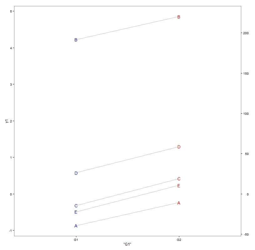
如果想要保存图片,则必须将调用包装到设备打开/关闭中:
png(...)
PlotWithFudgeAxis(tmpPlot, FudgeAxis)
dev.off()
p1 <-
  ggplot() + aes(mns)+ geom_histogram(aes(y=..density..), binwidth=0.01, colour="black", fill="white") + geom_vline(aes(xintercept=mean(mns, na.rm=T)), color="red", linetype="dashed", size=1) +  geom_density(alpha=.2)

p2 <-
  ggplot() + aes(mns)+ geom_histogram( binwidth=0.01, colour="black", fill="white") + geom_vline(aes(xintercept=mean(mns, na.rm=T)), color="red", linetype="dashed", size=1)

multiplot(p1,p2,cols=2)
multiplot拥有更多的选项/功能。https://dev59.com/F2sz5IYBdhLWcg3wTl4T#51220506/ - Tung对我来说最困难的部分是找出两个轴之间的转换函数。我使用了myCurveFit进行计算。
> dput(combined_80_8192 %>% filter (time > 270, time < 280))
structure(list(run = c(268L, 268L, 268L, 268L, 268L, 268L, 268L,
268L, 268L, 268L, 263L, 263L, 263L, 263L, 263L, 263L, 263L, 263L,
263L, 263L, 269L, 269L, 269L, 269L, 269L, 269L, 269L, 269L, 269L,
269L, 261L, 261L, 261L, 261L, 261L, 261L, 261L, 261L, 261L, 261L,
267L, 267L, 267L, 267L, 267L, 267L, 267L, 267L, 267L, 267L, 265L,
265L, 265L, 265L, 265L, 265L, 265L, 265L, 265L, 265L, 266L, 266L,
266L, 266L, 266L, 266L, 266L, 266L, 266L, 266L, 262L, 262L, 262L,
262L, 262L, 262L, 262L, 262L, 262L, 262L, 264L, 264L, 264L, 264L,
264L, 264L, 264L, 264L, 264L, 264L, 260L, 260L, 260L, 260L, 260L,
260L, 260L, 260L, 260L, 260L), repetition = c(8L, 8L, 8L, 8L,
8L, 8L, 8L, 8L, 8L, 8L, 3L, 3L, 3L, 3L, 3L, 3L, 3L, 3L, 3L, 3L,
9L, 9L, 9L, 9L, 9L, 9L, 9L, 9L, 9L, 9L, 1L, 1L, 1L, 1L, 1L, 1L,
1L, 1L, 1L, 1L, 7L, 7L, 7L, 7L, 7L, 7L, 7L, 7L, 7L, 7L, 5L, 5L,
5L, 5L, 5L, 5L, 5L, 5L, 5L, 5L, 6L, 6L, 6L, 6L, 6L, 6L, 6L, 6L,
6L, 6L, 2L, 2L, 2L, 2L, 2L, 2L, 2L, 2L, 2L, 2L, 4L, 4L, 4L, 4L,
4L, 4L, 4L, 4L, 4L, 4L, 0L, 0L, 0L, 0L, 0L, 0L, 0L, 0L, 0L, 0L
), module = structure(c(1L, 1L, 1L, 1L, 1L, 1L, 1L, 1L, 1L, 1L,
1L, 1L, 1L, 1L, 1L, 1L, 1L, 1L, 1L, 1L, 1L, 1L, 1L, 1L, 1L, 1L,
1L, 1L, 1L, 1L, 1L, 1L, 1L, 1L, 1L, 1L, 1L, 1L, 1L, 1L, 1L, 1L,
1L, 1L, 1L, 1L, 1L, 1L, 1L, 1L, 1L, 1L, 1L, 1L, 1L, 1L, 1L, 1L,
1L, 1L, 1L, 1L, 1L, 1L, 1L, 1L, 1L, 1L, 1L, 1L, 1L, 1L, 1L, 1L,
1L, 1L, 1L, 1L, 1L, 1L, 1L, 1L, 1L, 1L, 1L, 1L, 1L, 1L, 1L, 1L,
1L, 1L, 1L, 1L, 1L, 1L, 1L, 1L, 1L, 1L), .Label = "scenario.node[0].nicVLCTail.phyVLC", class = "factor"),
    configname = structure(c(1L, 1L, 1L, 1L, 1L, 1L, 1L, 1L,
    1L, 1L, 1L, 1L, 1L, 1L, 1L, 1L, 1L, 1L, 1L, 1L, 1L, 1L, 1L,
    1L, 1L, 1L, 1L, 1L, 1L, 1L, 1L, 1L, 1L, 1L, 1L, 1L, 1L, 1L,
    1L, 1L, 1L, 1L, 1L, 1L, 1L, 1L, 1L, 1L, 1L, 1L, 1L, 1L, 1L,
    1L, 1L, 1L, 1L, 1L, 1L, 1L, 1L, 1L, 1L, 1L, 1L, 1L, 1L, 1L,
    1L, 1L, 1L, 1L, 1L, 1L, 1L, 1L, 1L, 1L, 1L, 1L, 1L, 1L, 1L,
    1L, 1L, 1L, 1L, 1L, 1L, 1L, 1L, 1L, 1L, 1L, 1L, 1L, 1L, 1L,
    1L, 1L), .Label = "Road-Vlc", class = "factor"), packetByteLength = c(8192L,
    8192L, 8192L, 8192L, 8192L, 8192L, 8192L, 8192L, 8192L, 8192L,
    8192L, 8192L, 8192L, 8192L, 8192L, 8192L, 8192L, 8192L, 8192L,
    8192L, 8192L, 8192L, 8192L, 8192L, 8192L, 8192L, 8192L, 8192L,
    8192L, 8192L, 8192L, 8192L, 8192L, 8192L, 8192L, 8192L, 8192L,
    8192L, 8192L, 8192L, 8192L, 8192L, 8192L, 8192L, 8192L, 8192L,
    8192L, 8192L, 8192L, 8192L, 8192L, 8192L, 8192L, 8192L, 8192L,
    8192L, 8192L, 8192L, 8192L, 8192L, 8192L, 8192L, 8192L, 8192L,
    8192L, 8192L, 8192L, 8192L, 8192L, 8192L, 8192L, 8192L, 8192L,
    8192L, 8192L, 8192L, 8192L, 8192L, 8192L, 8192L, 8192L, 8192L,
    8192L, 8192L, 8192L, 8192L, 8192L, 8192L, 8192L, 8192L, 8192L,
    8192L, 8192L, 8192L, 8192L, 8192L, 8192L, 8192L, 8192L, 8192L
    ), numVehicles = c(2L, 2L, 2L, 2L, 2L, 2L, 2L, 2L, 2L, 2L,
    2L, 2L, 2L, 2L, 2L, 2L, 2L, 2L, 2L, 2L, 2L, 2L, 2L, 2L, 2L,
    2L, 2L, 2L, 2L, 2L, 2L, 2L, 2L, 2L, 2L, 2L, 2L, 2L, 2L, 2L,
    2L, 2L, 2L, 2L, 2L, 2L, 2L, 2L, 2L, 2L, 2L, 2L, 2L, 2L, 2L,
    2L, 2L, 2L, 2L, 2L, 2L, 2L, 2L, 2L, 2L, 2L, 2L, 2L, 2L, 2L,
    2L, 2L, 2L, 2L, 2L, 2L, 2L, 2L, 2L, 2L, 2L, 2L, 2L, 2L, 2L,
    2L, 2L, 2L, 2L, 2L, 2L, 2L, 2L, 2L, 2L, 2L, 2L, 2L, 2L, 2L
    ), dDistance = c(80L, 80L, 80L, 80L, 80L, 80L, 80L, 80L,
    80L, 80L, 80L, 80L, 80L, 80L, 80L, 80L, 80L, 80L, 80L, 80L,
    80L, 80L, 80L, 80L, 80L, 80L, 80L, 80L, 80L, 80L, 80L, 80L,
    80L, 80L, 80L, 80L, 80L, 80L, 80L, 80L, 80L, 80L, 80L, 80L,
    80L, 80L, 80L, 80L, 80L, 80L, 80L, 80L, 80L, 80L, 80L, 80L,
    80L, 80L, 80L, 80L, 80L, 80L, 80L, 80L, 80L, 80L, 80L, 80L,
    80L, 80L, 80L, 80L, 80L, 80L, 80L, 80L, 80L, 80L, 80L, 80L,
    80L, 80L, 80L, 80L, 80L, 80L, 80L, 80L, 80L, 80L, 80L, 80L,
    80L, 80L, 80L, 80L, 80L, 80L, 80L, 80L), time = c(270.166006903445,
    271.173853699836, 272.175873251122, 273.177524313334, 274.182946177105,
    275.188959464989, 276.189675339937, 277.198250244799, 278.204619457189,
    279.212562800009, 270.164199199177, 271.168527215152, 272.173072994958,
    273.179210429715, 274.184351047337, 275.18980754378, 276.194816792995,
    277.198598277809, 278.202398083519, 279.210634593917, 270.210674322891,
    271.212395107473, 272.218871923292, 273.219060500457, 274.220486359614,
    275.22401452372, 276.229646658839, 277.231060448138, 278.240407241942,
    279.2437126347, 270.283554249858, 271.293168593832, 272.298574288769,
    273.304413221348, 274.306272082517, 275.309023049011, 276.317805897347,
    277.324403550028, 278.332855848701, 279.334046374594, 270.118608539613,
    271.127947700074, 272.133887145863, 273.135726000491, 274.135994529981,
    275.136563912708, 276.140120735361, 277.144298344151, 278.146885137621,
    279.147552358659, 270.206015567272, 271.214618077209, 272.216566814903,
    273.225435592582, 274.234014573683, 275.242949179958, 276.248417809711,
    277.248800670023, 278.249750333404, 279.252926560188, 270.217182684494,
    271.218357511397, 272.224698488895, 273.231112784327, 274.238740508457,
    275.242715184122, 276.249053562718, 277.250325509798, 278.258488063493,
    279.261141590137, 270.282904173953, 271.284689544638, 272.294220723234,
    273.299749415592, 274.30628880553, 275.312075103126, 276.31579134717,
    277.321905523606, 278.326305136748, 279.333056502253, 270.258991527456,
    271.260224091407, 272.270076810133, 273.27052037648, 274.274119348094,
    275.280808254502, 276.286353887245, 277.287064312339, 278.294444793276,
    279.296772014594, 270.333066283904, 271.33877455992, 272.345842319903,
    273.350858180493, 274.353972278505, 275.360454510107, 276.365088896161,
    277.369166956941, 278.372571708911, 279.38017503079), distanceToTx = c(80.255266401689,
    80.156059067023, 79.98823695539, 79.826647129071, 79.76678667135,
    79.788239825292, 79.734539327997, 79.74766421514, 79.801243848241,
    79.765920888341, 80.255266401689, 80.15850240049, 79.98823695539,
    79.826647129071, 79.76678667135, 79.788239825292, 79.735078924078,
    79.74766421514, 79.801243848241, 79.764622734914, 80.251248121732,
    80.146436869316, 79.984682320466, 79.82292012342, 79.761908518748,
    79.796988776281, 79.736920997657, 79.745038376718, 79.802638836686,
    79.770029970452, 80.243475525691, 80.127918207499, 79.978303140866,
    79.816259117883, 79.749322030693, 79.809916018889, 79.744456560867,
    79.738655068783, 79.788697533211, 79.784288359619, 80.260412958482,
    80.168426829066, 79.992034911214, 79.830845773284, 79.7756751763,
    79.778156038931, 79.732399593756, 79.752769548846, 79.799967731078,
    79.757585110481, 80.251248121732, 80.146436869316, 79.984682320466,
    79.822062073459, 79.75884601899, 79.801590491435, 79.738335109094,
    79.74347007248, 79.803215965043, 79.771471198955, 80.250257298678,
    80.146436869316, 79.983831684476, 79.822062073459, 79.75884601899,
    79.801590491435, 79.738335109094, 79.74347007248, 79.803849157574,
    79.771471198955, 80.243475525691, 80.130180105198, 79.978303140866,
    79.816881283718, 79.749322030693, 79.80984572883, 79.744456560867,
    79.738655068783, 79.790548644175, 79.784288359619, 80.246349000313,
    80.137056554491, 79.980581246037, 79.818924707937, 79.753176142361,
    79.808777040341, 79.741609845588, 79.740770913572, 79.796316397253,
    79.777593733292, 80.238796415443, 80.119021911134, 79.974810568944,
    79.814065350562, 79.743657315504, 79.810146783217, 79.749945098869,
    79.737122584544, 79.781650522348, 79.791554933936), headerNoError = c(0.99999999989702,
    0.9999999999981, 0.99999999999946, 0.9999999928026, 0.99999873265475,
    0.77080141574964, 0.99007491438593, 0.99994396605059, 0.45588747062284,
    0.93484381262491, 0.99999999989702, 0.99999999999816, 0.99999999999946,
    0.9999999928026, 0.99999873265475, 0.77080141574964, 0.99008458785106,
    0.99994396605059, 0.45588747062284, 0.93480223051707, 0.99999999989735,
    0.99999999999789, 0.99999999999946, 0.99999999287551, 0.99999876302649,
    0.46903147501117, 0.98835168988253, 0.99994427085086, 0.45235035271542,
    0.93496741877335, 0.99999999989803, 0.99999999999781, 0.99999999999948,
    0.99999999318224, 0.99994254156311, 0.46891362282273, 0.93382613917348,
    0.99994594904099, 0.93002915596843, 0.93569767251247, 0.99999999989658,
    0.99999999998074, 0.99999999999946, 0.99999999272802, 0.99999871586781,
    0.76935240919896, 0.99002587758346, 0.99999881589732, 0.46179415706093,
    0.93417422376389, 0.99999999989735, 0.99999999999789, 0.99999999999946,
    0.99999999289347, 0.99999876940486, 0.46930769326427, 0.98837353639905,
    0.99994447154714, 0.16313586712094, 0.93500824170148, 0.99999999989744,
    0.99999999999789, 0.99999999999946, 0.99999999289347, 0.99999876940486,
    0.46930769326427, 0.98837353639905, 0.99994447154714, 0.16330039178981,
    0.93500824170148, 0.99999999989803, 0.99999999999781, 0.99999999999948,
    0.99999999316541, 0.99994254156311, 0.46794586553266, 0.93382613917348,
    0.99994594904099, 0.9303627789484, 0.93569767251247, 0.99999999989778,
    0.9999999999978, 0.99999999999948, 0.99999999311433, 0.99999878195152,
    0.47101897739483, 0.93368891853679, 0.99994556595217, 0.7571113417265,
    0.93553999975802, 0.99999999998191, 0.99999999999784, 0.99999999999971,
    0.99999891129658, 0.99994309267792, 0.46510628979591, 0.93442584181035,
    0.99894450514543, 0.99890078483692, 0.76933812306423), receivedPower_dbm = c(-93.023492290586,
    -92.388378035287, -92.205716340607, -93.816400586752, -95.023489422885,
    -100.86308557253, -98.464763536915, -96.175707680373, -102.06189538385,
    -99.716653422746, -93.023492290586, -92.384760627397, -92.205716340607,
    -93.816400586752, -95.023489422885, -100.86308557253, -98.464201120719,
    -96.175707680373, -102.06189538385, -99.717150021506, -93.022927803442,
    -92.404017215549, -92.204561341714, -93.814319484729, -95.016990717792,
    -102.01669022332, -98.558088145955, -96.173817001483, -102.07406915124,
    -99.71517574876, -93.021813165972, -92.409586309743, -92.20229160243,
    -93.805335867418, -96.184419849593, -102.01709540787, -99.728735187547,
    -96.163233028048, -99.772547164798, -99.706399753853, -93.024204617071,
    -92.745813384859, -92.206884754512, -93.818508150122, -95.027018807793,
    -100.87000577258, -98.467607232407, -95.005311380324, -102.04157607608,
    -99.724619517, -93.022927803442, -92.404017215549, -92.204561341714,
    -93.813803344588, -95.015606885523, -102.0157405687, -98.556982278361,
    -96.172566862738, -103.21871579865, -99.714687230796, -93.022787428238,
    -92.404017215549, -92.204274688493, -93.813803344588, -95.015606885523,
    -102.0157405687, -98.556982278361, -96.172566862738, -103.21784988098,
    -99.714687230796, -93.021813165972, -92.409950613665, -92.20229160243,
    -93.805838770576, -96.184419849593, -102.02042267497, -99.728735187547,
    -96.163233028048, -99.768774335378, -99.706399753853, -93.022228914406,
    -92.411048503835, -92.203136463155, -93.807357409082, -95.012865008237,
    -102.00985717796, -99.730352912911, -96.165675535906, -100.92744056572,
    -99.708301333236, -92.735781110993, -92.408137395049, -92.119533319039,
    -94.982938427575, -96.181073124017, -102.03018610927, -99.721633629806,
    -97.32940323644, -97.347613268692, -100.87007386786), snr = c(49.848348091678,
    57.698190927109, 60.17669971462, 41.529809724535, 31.452202106925,
    8.1976890851341, 14.240447804094, 24.122884195464, 6.2202875499406,
    10.674183333671, 49.848348091678, 57.746270018264, 60.17669971462,
    41.529809724535, 31.452202106925, 8.1976890851341, 14.242292077376,
    24.122884195464, 6.2202875499406, 10.672962852322, 49.854827699773,
    57.49079026127, 60.192705735317, 41.549715223147, 31.499301851462,
    6.2853718719014, 13.937702343688, 24.133388256416, 6.2028757927148,
    10.677815810561, 49.867624820879, 57.417115267867, 60.224172277442,
    41.635752021705, 24.074540962859, 6.2847854917092, 10.644529778044,
    24.19227425387, 10.537686730745, 10.699414795917, 49.84017267426,
    53.139646558768, 60.160512118809, 41.509660845114, 31.42665220053,
    8.1846370024428, 14.231126423354, 31.584125885363, 6.2494585568733,
    10.654622041348, 49.854827699773, 57.49079026127, 60.192705735317,
    41.55465351989, 31.509340361646, 6.2867464196657, 13.941251828322,
    24.140336174865, 4.765718874642, 10.679016976694, 49.856439162736,
    57.49079026127, 60.196678846453, 41.55465351989, 31.509340361646,
    6.2867464196657, 13.941251828322, 24.140336174865, 4.7666691818074,
    10.679016976694, 49.867624820879, 57.412299088098, 60.224172277442,
    41.630930975211, 24.074540962859, 6.279972363168, 10.644529778044,
    24.19227425387, 10.546845071479, 10.699414795917, 49.862851240855,
    57.397787176282, 60.212457625018, 41.61637603957, 31.529239767749,
    6.2952688513108, 10.640565481982, 24.178672145334, 8.0771089950663,
    10.694731030907, 53.262541905639, 57.43627424514, 61.382796189332,
    31.747253311549, 24.093100244121, 6.2658701281075, 10.661949889074,
    18.495227442305, 18.417839037171, 8.1845086722809), frameId = c(15051,
    15106, 15165, 15220, 15279, 15330, 15385, 15452, 15511, 15566,
    15019, 15074, 15129, 15184, 15239, 15298, 15353, 15412, 15471,
    15526, 14947, 14994, 15057, 15112, 15171, 15226, 15281, 15332,
    15391, 15442, 14971, 15030, 15085, 15144, 15203, 15262, 15321,
    15380, 15435, 15490, 14915, 14978, 15033, 15092, 15147, 15198,
    15257, 15312, 15371, 15430, 14975, 15034, 15089, 15140, 15195,
    15254, 15313, 15368, 15427, 15478, 14987, 15046, 15105, 15160,
    15215, 15274, 15329, 15384, 15447, 15506, 14943, 15002, 15061,
    15116, 15171, 15230, 15285, 15344, 15399, 15454, 14971, 15026,
    15081, 15136, 15195, 15258, 15313, 15368, 15423, 15478, 15039,
    15094, 15149, 15204, 15263, 15314, 15369, 15428, 15487, 15546
    ), packetOkSinr = c(0.99999999314881, 0.9999999998736, 0.99999999996428,
    0.99999952114066, 0.99991568416005, 3.00628034688444e-08,
    0.51497487795954, 0.99627877136019, 0, 0.011303253101957,
    0.99999999314881, 0.99999999987726, 0.99999999996428, 0.99999952114066,
    0.99991568416005, 3.00628034688444e-08, 0.51530974419663,
    0.99627877136019, 0, 0.011269851265775, 0.9999999931708,
    0.99999999985986, 0.99999999996428, 0.99999952599145, 0.99991770469509,
    0, 0.45861812482641, 0.99629897628155, 0, 0.011403119534097,
    0.99999999321568, 0.99999999985437, 0.99999999996519, 0.99999954639936,
    0.99618434878558, 0, 0.010513119213425, 0.99641022914441,
    0.00801687746446111, 0.012011103529927, 0.9999999931195,
    0.99999999871861, 0.99999999996428, 0.99999951617905, 0.99991456738049,
    2.6525298291169e-08, 0.51328066587104, 0.9999212220316, 0,
    0.010777054258914, 0.9999999931708, 0.99999999985986, 0.99999999996428,
    0.99999952718674, 0.99991812902805, 0, 0.45929307038653,
    0.99631228046814, 0, 0.011436292559188, 0.99999999317629,
    0.99999999985986, 0.99999999996428, 0.99999952718674, 0.99991812902805,
    0, 0.45929307038653, 0.99631228046814, 0, 0.011436292559188,
    0.99999999321568, 0.99999999985437, 0.99999999996519, 0.99999954527918,
    0.99618434878558, 0, 0.010513119213425, 0.99641022914441,
    0.00821047996950475, 0.012011103529927, 0.99999999319919,
    0.99999999985345, 0.99999999996519, 0.99999954188106, 0.99991896371849,
    0, 0.010410830482692, 0.996384831822, 9.12484388049251e-09,
    0.011877185067536, 0.99999999879646, 0.9999999998562, 0.99999999998077,
    0.99992756868677, 0.9962208785486, 0, 0.010971897073662,
    0.93214999078663, 0.92943956665979, 2.64925478221656e-08),
    snir = c(49.848348091678, 57.698190927109, 60.17669971462,
    41.529809724535, 31.452202106925, 8.1976890851341, 14.240447804094,
    24.122884195464, 6.2202875499406, 10.674183333671, 49.848348091678,
    57.746270018264, 60.17669971462, 41.529809724535, 31.452202106925,
    8.1976890851341, 14.242292077376, 24.122884195464, 6.2202875499406,
    10.672962852322, 49.854827699773, 57.49079026127, 60.192705735317,
    41.549715223147, 31.499301851462, 6.2853718719014, 13.937702343688,
    24.133388256416, 6.2028757927148, 10.677815810561, 49.867624820879,
    57.417115267867, 60.224172277442, 41.635752021705, 24.074540962859,
    6.2847854917092, 10.644529778044, 24.19227425387, 10.537686730745,
    10.699414795917, 49.84017267426, 53.139646558768, 60.160512118809,
    41.509660845114, 31.42665220053, 8.1846370024428, 14.231126423354,
    31.584125885363, 6.2494585568733, 10.654622041348, 49.854827699773,
    57.49079026127, 60.192705735317, 41.55465351989, 31.509340361646,
    6.2867464196657, 13.941251828322, 24.140336174865, 4.765718874642,
    10.679016976694, 49.856439162736, 57.49079026127, 60.196678846453,
    41.55465351989, 31.509340361646, 6.2867464196657, 13.941251828322,
    24.140336174865, 4.7666691818074, 10.679016976694, 49.867624820879,
    57.412299088098, 60.224172277442, 41.630930975211, 24.074540962859,
    6.279972363168, 10.644529778044, 24.19227425387, 10.546845071479,
    10.699414795917, 49.862851240855, 57.397787176282, 60.212457625018,
    41.61637603957, 31.529239767749, 6.2952688513108, 10.640565481982,
    24.178672145334, 8.0771089950663, 10.694731030907, 53.262541905639,
    57.43627424514, 61.382796189332, 31.747253311549, 24.093100244121,
    6.2658701281075, 10.661949889074, 18.495227442305, 18.417839037171,
    8.1845086722809), ookSnirBer = c(8.8808636558081e-24, 3.2219795637026e-27,
    2.6468895519653e-28, 3.9807779074715e-20, 1.0849324265615e-15,
    2.5705217057696e-05, 4.7313805615763e-08, 1.8800438086075e-12,
    0.00021005320203921, 1.9147343768384e-06, 8.8808636558081e-24,
    3.0694773489537e-27, 2.6468895519653e-28, 3.9807779074715e-20,
    1.0849324265615e-15, 2.5705217057696e-05, 4.7223753038869e-08,
    1.8800438086075e-12, 0.00021005320203921, 1.9171738578051e-06,
    8.8229427230445e-24, 3.9715925056443e-27, 2.6045198111088e-28,
    3.9014083702734e-20, 1.0342658440386e-15, 0.00019591630514278,
    6.4692014108683e-08, 1.8600094209271e-12, 0.0002140067535655,
    1.9074922485477e-06, 8.7096574467175e-24, 4.2779443633862e-27,
    2.5231916788231e-28, 3.5761615214425e-20, 1.9750692814982e-12,
    0.0001960392878411, 1.9748966344895e-06, 1.7515881895994e-12,
    2.2078334799411e-06, 1.8649940680806e-06, 8.954486301678e-24,
    3.2021085732779e-25, 2.690441113724e-28, 4.0627628846548e-20,
    1.1134484878561e-15, 2.6061691733331e-05, 4.777159157954e-08,
    9.4891388749738e-16, 0.00020359398491544, 1.9542110660398e-06,
    8.8229427230445e-24, 3.9715925056443e-27, 2.6045198111088e-28,
    3.8819641115984e-20, 1.0237769828158e-15, 0.00019562832342849,
    6.4455095380046e-08, 1.8468752030971e-12, 0.0010099091367628,
    1.9051035165106e-06, 8.8085966897635e-24, 3.9715925056443e-27,
    2.594108048185e-28, 3.8819641115984e-20, 1.0237769828158e-15,
    0.00019562832342849, 6.4455095380046e-08, 1.8468752030971e-12,
    0.0010088638355194, 1.9051035165106e-06, 8.7096574467175e-24,
    4.2987746909572e-27, 2.5231916788231e-28, 3.593647329558e-20,
    1.9750692814982e-12, 0.00019705170257492, 1.9748966344895e-06,
    1.7515881895994e-12, 2.1868296425817e-06, 1.8649940680806e-06,
    8.7517439682173e-24, 4.3621551072316e-27, 2.553168170837e-28,
    3.6469582463164e-20, 1.0032983660212e-15, 0.00019385229409318,
    1.9830820164805e-06, 1.7760568361323e-12, 2.919419915209e-05,
    1.8741284335866e-06, 2.8285944348148e-25, 4.1960751547207e-27,
    7.8468215407139e-29, 8.0407329049747e-16, 1.9380328071065e-12,
    0.00020004849911333, 1.9393279417733e-06, 5.9354475879597e-10,
    6.4258355913627e-10, 2.6065221215415e-05), ookSnrBer = c(8.8808636558081e-24,
    3.2219795637026e-27, 2.6468895519653e-28, 3.9807779074715e-20,
    1.0849324265615e-15, 2.5705217057696e-05, 4.7313805615763e-08,
    1.8800438086075e-12, 0.00021005320203921, 1.9147343768384e-06,
    8.8808636558081e-24, 3.0694773489537e-27, 2.6468895519653e-28,
    3.9807779074715e-20, 1.0849324265615e-15, 2.5705217057696e-05,
    4.7223753038869e-08, 1.8800438086075e-12, 0.00021005320203921,
    1.9171738578051e-06, 8.8229427230445e-24, 3.9715925056443e-27,
    2.6045198111088e-28, 3.9014083702734e-20, 1.0342658440386e-15,
    0.00019591630514278, 6.4692014108683e-08, 1.8600094209271e-12,
    0.0002140067535655, 1.9074922485477e-06, 8.7096574467175e-24,
    4.2779443633862e-27, 2.5231916788231e-28, 3.5761615214425e-20,
    1.9750692814982e-12, 0.0001960392878411, 1.9748966344895e-06,
    1.7515881895994e-12, 2.2078334799411e-06, 1.8649940680806e-06,
    8.954486301678e-24, 3.2021085732779e-25, 2.690441113724e-28,
    4.0627628846548e-20, 1.1134484878561e-15, 2.6061691733331e-05,
    4.777159157954e-08, 9.4891388749738e-16, 0.00020359398491544,
    1.9542110660398e-06, 8.8229427230445e-24, 3.9715925056443e-27,
    2.6045198111088e-28, 3.8819641115984e-20, 1.0237769828158e-15,
    0.00019562832342849, 6.4455095380046e-08, 1.8468752030971e-12,
    0.0010099091367628, 1.9051035165106e-06, 8.8085966897635e-24,
    3.9715925056443e-27, 2.594108048185e-28, 3.8819641115984e-20,
    1.0237769828158e-15, 0.00019562832342849, 6.4455095380046e-08,
    1.8468752030971e-12, 0.0010088638355194, 1.9051035165106e-06,
    8.7096574467175e-24, 4.2987746909572e-27, 2.5231916788231e-28,
    3.593647329558e-20, 1.9750692814982e-12, 0.00019705170257492,
    1.9748966344895e-06, 1.7515881895994e-12, 2.1868296425817e-06,
    1.8649940680806e-06, 8.7517439682173e-24, 4.3621551072316e-27,
    2.553168170837e-28, 3.6469582463164e-20, 1.0032983660212e-15,
    0.00019385229409318, 1.9830820164805e-06, 1.7760568361323e-12,
    2.919419915209e-05, 1.8741284335866e-06, 2.8285944348148e-25,
    4.1960751547207e-27, 7.8468215407139e-29, 8.0407329049747e-16,
    1.9380328071065e-12, 0.00020004849911333, 1.9393279417733e-06,
    5.9354475879597e-10, 6.4258355913627e-10, 2.6065221215415e-05
    )), class = "data.frame", row.names = c(NA, -100L), .Names = c("run",
"repetition", "module", "configname", "packetByteLength", "numVehicles",
"dDistance", "time", "distanceToTx", "headerNoError", "receivedPower_dbm",
"snr", "frameId", "packetOkSinr", "snir", "ookSnirBer", "ookSnrBer"
))
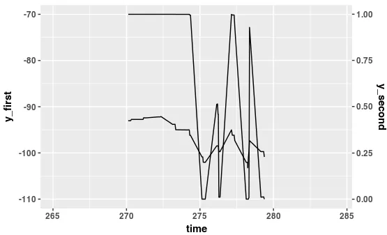
查找转换函数
转换函数: f(y1) = 0.025*x + 2.75
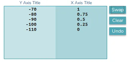
转换函数: f(y1) = 40*x - 110
绘图
请注意在ggplot调用中如何使用转换函数即时转换数据。
ggplot(data=combined_80_8192 %>% filter (time > 270, time < 280), aes(x=time) ) +
  stat_summary(aes(y=receivedPower_dbm ), fun.y=mean, geom="line", colour="black") +
  stat_summary(aes(y=packetOkSinr*40 - 110 ), fun.y=mean, geom="line", colour="black", position = position_dodge(width=10)) +
  scale_x_continuous() +
  scale_y_continuous(breaks = seq(-0,-110,-10), "y_first", sec.axis=sec_axis(~.*0.025+2.75, name="y_second") )
stat_summary 调用为第一个 y 轴设置基础。
第二个 stat_summary 调用被称为数据转换。请记住,所有数据都将以第一个 y 轴为基础。因此,需要对第一个 y 轴进行归一化处理。为此,我在数据上使用了转换函数:y=packetOkSinr*40 - 110
现在,为了转换第二个轴,我在 scale_y_continuous 调用中使用相反的函数:sec.axis=sec_axis(~.*0.025+2.75, name="y_second")。
coef(lm(c(-70, -110) ~ c(1,0)))和coef(lm(c(1,0) ~ c(-70, -110)))。您可以定义一个辅助函数,例如equationise <- function(range = c(-70, -110), target = c(1,0)){ c = coef(lm(target ~ range)) as.formula(substitute(~ a*. + b, list(a=c[[2]], b=c[[1]]))) } - baptiste
scale_y_*中已经被称为sec.axis的本地ggplot2实现。 - PatrickT