如果我使用Python中的seaborn库绘制线性回归结果,有没有办法找出回归的数字结果?例如,我可能想知道拟合系数或拟合的R2值。
我可以使用底层statsmodels接口重新运行相同的拟合,但这似乎是不必要的重复努力,并且我想能够比较所得到的系数以确保数值结果与我在图表中看到的结果相同。
我可以使用底层statsmodels接口重新运行相同的拟合,但这似乎是不必要的重复努力,并且我想能够比较所得到的系数以确保数值结果与我在图表中看到的结果相同。
这是无法做到的。
在我看来,让一种可视化库提供统计建模结果是反过来的。建模库 statsmodels 允许您拟合模型,然后绘制与您拟合的模型完全对应的图形。如果您想要确切的对应关系,我认为这种操作顺序更有意义。
您可能会说,“但是 statsmodels 中的图形选项不如 seaborn 多。” 但我认为这很有道理 - statsmodels 是一种建模库,有时使用可视化来服务于建模。 seaborn 是一种可视化库,有时使用建模来服务于可视化。专业化是好的,试图做所有事情是不好的。
幸运的是,seaborn 和 statsmodels 都使用整洁数据。这意味着您实际上需要非常少的重复工作,就可以通过适当的工具获得两者的图形和模型。
Seaborn的创作者不幸地表示,他不会添加这样的功能。以下是一些选项。(最后一节包含了我的原始建议,它使用了seaborn的私有实现细节,并不特别灵活。)
regplot的简单替代版本下面的函数在散点图上叠加拟合线,并返回statsmodels的结果。这支持sns.regplot最简单、也许是最常见的用法,但没有实现任何更高级的功能。
import statsmodels.api as sm


def simple_regplot(
    x, y, n_std=2, n_pts=100, ax=None, scatter_kws=None, line_kws=None, ci_kws=None
):
    """ Draw a regression line with error interval. """
    ax = plt.gca() if ax is None else ax

    # calculate best-fit line and interval
    x_fit = sm.add_constant(x)
    fit_results = sm.OLS(y, x_fit).fit()

    eval_x = sm.add_constant(np.linspace(np.min(x), np.max(x), n_pts))
    pred = fit_results.get_prediction(eval_x)

    # draw the fit line and error interval
    ci_kws = {} if ci_kws is None else ci_kws
    ax.fill_between(
        eval_x[:, 1],
        pred.predicted_mean - n_std * pred.se_mean,
        pred.predicted_mean + n_std * pred.se_mean,
        alpha=0.5,
        **ci_kws,
    )
    line_kws = {} if line_kws is None else line_kws
    h = ax.plot(eval_x[:, 1], pred.predicted_mean, **line_kws)

    # draw the scatterplot
    scatter_kws = {} if scatter_kws is None else scatter_kws
    ax.scatter(x, y, c=h[0].get_color(), **scatter_kws)

    return fit_results
statsmodels 的结果包含大量信息,例如:
>>> print(fit_results.summary())

                            OLS Regression Results
==============================================================================
Dep. Variable:                      y   R-squared:                       0.477
Model:                            OLS   Adj. R-squared:                  0.471
Method:                 Least Squares   F-statistic:                     89.23
Date:                Fri, 08 Jan 2021   Prob (F-statistic):           1.93e-15
Time:                        17:56:00   Log-Likelihood:                -137.94
No. Observations:                 100   AIC:                             279.9
Df Residuals:                      98   BIC:                             285.1
Df Model:                           1
Covariance Type:            nonrobust
==============================================================================
                 coef    std err          t      P>|t|      [0.025      0.975]
------------------------------------------------------------------------------
const         -0.1417      0.193     -0.735      0.464      -0.524       0.241
x1             3.1456      0.333      9.446      0.000       2.485       3.806
==============================================================================
Omnibus:                        2.200   Durbin-Watson:                   1.777
Prob(Omnibus):                  0.333   Jarque-Bera (JB):                1.518
Skew:                          -0.002   Prob(JB):                        0.468
Kurtosis:                       2.396   Cond. No.                         4.35
==============================================================================

Notes:
[1] Standard Errors assume that the covariance matrix of the errors is correctly specified.
与下面的原始答案相比,上述方法的优点在于它很容易扩展到更复杂的拟合。
厚颜无耻地插一下: 这是我编写的一个扩展的regplot函数,实现了sns.regplot的大部分功能: https://github.com/ttesileanu/pydove。
虽然还有一些功能尚未实现,但我编写的函数
statsmodels计算置信区间,而不是使用自助法。log(x)中的多项式)。Seaborn的创建者不幸地表示他不会添加这样的功能,所以这是一个解决方法。
def regplot(
    *args,
    line_kws=None,
    marker=None,
    scatter_kws=None,
    **kwargs
):
    # this is the class that `sns.regplot` uses
    plotter = sns.regression._RegressionPlotter(*args, **kwargs)

    # this is essentially the code from `sns.regplot`
    ax = kwargs.get("ax", None)
    if ax is None:
        ax = plt.gca()

    scatter_kws = {} if scatter_kws is None else copy.copy(scatter_kws)
    scatter_kws["marker"] = marker
    line_kws = {} if line_kws is None else copy.copy(line_kws)

    plotter.plot(ax, scatter_kws, line_kws)

    # unfortunately the regression results aren't stored, so we rerun
    grid, yhat, err_bands = plotter.fit_regression(plt.gca())

    # also unfortunately, this doesn't return the parameters, so we infer them
    slope = (yhat[-1] - yhat[0]) / (grid[-1] - grid[0])
    intercept = yhat[0] - slope * grid[0]
    return slope, intercept
seaborn自己的回归类,因此结果保证与所显示的一致。当然,缺点是我们使用了seaborn中的私有实现细节,这可能会在任何时候发生故障。local variable 'scatter_kws' referenced before assignment - 我该怎么解决? - Marioanzasdef中缺少了一些关键字参数。现在应该可以工作了,感谢@Marioanzas指出这一点! - Legendre17if 'alpha' in ci_kws: alpha = ci_kws['alpha'] del ci_kws['alpha'] else: alpha= 0.5 - Exiseaborn 更兼容。 - Legendre17很遗憾,直接从 seaborn.regplot 中提取数值信息是不可能的。因此,下面这个简单的函数拟合了一个多项式回归,并返回平滑线和相应置信区间的值。
import numpy as np
from scipy import stats

def polynomial_regression(X, y, order=1, confidence=95, num=100):
    confidence = 1 - ((1 - (confidence / 100)) / 2)
    y_model = np.polyval(np.polyfit(X, y, order), X)
    residual = y - y_model
    n = X.size
    m = 2
    dof = n - m
    t = stats.t.ppf(confidence, dof)
    std_error = (np.sum(residual**2) / dof)**.5
    X_line = np.linspace(np.min(X), np.max(X), num)
    y_line = np.polyval(np.polyfit(X, y, order), X_line)
    ci = t * std_error * (1/n + (X_line - np.mean(X))**2 / np.sum((X - np.mean(X))**2))**.5
    return X_line, y_line, ci
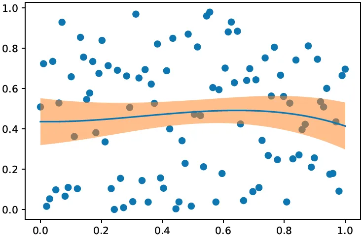
示例运行:
X = np.linspace(0,1,100)
y = np.random.random(100)

X_line, y_line, ci = polynomial_regression(X, y, order=3)

plt.scatter(X, y)
plt.plot(X_line, y_line)
plt.fill_between(X_line, y_line - ci, y_line + ci, alpha=.5)
浏览目前可用的文档,我发现使用scipy.stats.pearsonr模块可能是实现此功能的最接近方法。
r2 = stats.pearsonr("pct", "rdiff", df)
尝试在Pandas数据帧内直接运行时,由于违反了基本的scipy输入要求,会出现错误:
TypeError: pearsonr() takes exactly 2 arguments (3 given)
我找到了另一个使用Pandas Seaborn的用户,显然已经解决了这个问题:https://github.com/scipy/scipy/blob/v0.14.0/scipy/stats/stats.py#L2392
sns.regplot("rdiff", "pct", df, corr_func=stats.pearsonr);
但是,不幸的是我还没有成功让它工作,因为似乎作者创建了自己定制的“corr_func”,或者存在一个不公开的Seaborn参数传递方法,需要使用更加手动的方法:
# x and y should have same length.
    x = np.asarray(x)
    y = np.asarray(y)
    n = len(x)
    mx = x.mean()
    my = y.mean()
    xm, ym = x-mx, y-my
    r_num = np.add.reduce(xm * ym)
    r_den = np.sqrt(ss(xm) * ss(ym))
    r = r_num / r_den

# Presumably, if abs(r) > 1, then it is only some small artifact of floating
# point arithmetic.
r = max(min(r, 1.0), -1.0)
df = n-2
if abs(r) == 1.0:
    prob = 0.0
else:
    t_squared = r*r * (df / ((1.0 - r) * (1.0 + r)))
    prob = betai(0.5*df, 0.5, df / (df + t_squared))
return r, prob
希望这能推动原始请求向中间解决方案的进展,因为有很多需要的实用程序可以将回归适应度统计信息添加到Seaborn包中,以替代可以轻松从MS-Excel或股票Matplotlib lineplot中获得的内容。