geom_smooth自定义线性模型

Question

在查看这个问题时，我无法为geom_smooth指定自定义线性模型。 我的代码如下：

example.label <- c("A","A","A","A","A","B","B","B","B","B")
example.value <- c(5, 4, 4, 5, 3, 8, 9, 11, 10, 9)
example.age <- c(30, 40, 50, 60, 70, 30, 40, 50, 60, 70)
example.score <- c(90,95,89,91,85,83,88,94,83,90)
example.data <- data.frame(example.label, example.value,example.age,example.score)

p = ggplot(example.data, aes(x=example.age,
                         y=example.value,color=example.label)) +
  geom_point()
  #geom_smooth(method = lm)

cf = function(dt){
  lm(example.value ~example.age+example.score, data = dt)
}

cf(example.data)

p_smooth <- by(example.data, example.data$example.label, 
               function(x) geom_smooth(data=x, method = lm, formula = cf(x)))

p + p_smooth 

我遇到了这个错误/警告：

Warning messages:
1: Computation failed in `stat_smooth()`:
object 'weight' not found 
2: Computation failed in `stat_smooth()`:
object 'weight' not found 

我为什么会得到这个？如何正确指定自定义模型给 geom_smooth 方法。谢谢。

- AK88

---

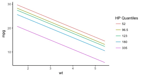
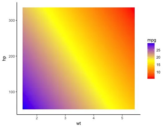
我认为 geom_smooth 的模型公式只能以 y ~ f(x) 的形式表示（例如，y ~ x 是默认的，或者 y ~ poly(x, 2)、 y ~ bs(x, df=4)等）。公式只能包括 x 和 y，它们将代表您传递给aes作为绘图 x 和 y 美学的任何数据列。如果您想绘制多元回归的结果，您可以构建一个数据框传递给 predict，然后使用例如 geom_line 绘制输出。 - eipi10

你认为值得尝试重新塑造数据，然后使用单列作为“x”和“subset”函数吗？ - AK88

这并不是重塑的问题。你真正能够用geom_smooth做的就是绘制包括y和x美学变量以及任何分类美学变量（例如颜色、形状）在内的回归。例如，在你的情况下，你可以做p + geom_smooth(method=lm, formula=y ~ poly(x, 2))或者p + geom_smooth(method=lm, formula=y ~ splines::bs(x, df=4))（尽管你需要更多的数据来理解后者）。这将为每个example.label级别提供单独的回归线。 - eipi10

例如，对于mtcars数据框，这里是mpg与wt的回归线，但按vs和am的级别进行分类：ggplot（mtcars，aes（wt，mpg，colour = interaction(vs，am，sep =“_”）））+ geom_point（）+ geom_smooth（se = FALSE，method =“lm”）。 - eipi10

我明白了，谢谢。看起来没有解决办法... - AK88

我已经添加了一个答案来扩展在评论中讨论的问题。 - eipi10

Answer 1

具有两个连续预测变量和一个连续结果的回归模型的回归函数存在于 3D 空间中（两个用于预测的维度和一个用于结果的维度），而 ggplot 图表是 2D 空间（一个连续预测变量在 x 轴上，结果在 y 轴上）。这就是为什么你不能使用 geom_smooth 绘制两个连续预测变量的函数的根本原因。

一种“解决办法”是选择一些特定值作为其中一个连续预测变量的值，然后为第二个连续预测变量在 x 轴上的每个选定值绘制一条线。

以下是使用 mtcars 数据框的示例。下面的回归模型使用 wt 和 hp 预测 mpg。我们然后绘制 mpg 对各个 hp 值下的 wt 的预测值。我们创建了一个预测数据框，然后使用 geom_line 绘制。图表中的每条线表示不同 hp 值下的 mpg 对 wt 的回归预测。当然，也可以颠倒 wt 和 hp 的角色。

library(ggplot)
theme_set(theme_classic())

d = mtcars
m2 = lm(mpg ~ wt + hp, data=d)

pred.data = expand.grid(wt = seq(min(d$wt), max(d$wt), length=20),
                        hp = quantile(d$hp))
pred.data$mpg = predict(m2, newdata=pred.data)

ggplot(pred.data, aes(wt, mpg, colour=factor(hp))) +
  geom_line() +
  labs(colour="HP Quantiles")

另一种选项是使用颜色渐变来表示mpg（结果），并将wt和hp绘制在x轴和y轴上：

pred.data = expand.grid(wt = seq(min(d$wt), max(d$wt), length=100),
                        hp = seq(min(d$hp), max(d$hp), length=100))
pred.data$mpg = predict(m2, newdata=pred.data)

ggplot(pred.data, aes(wt, hp, z=mpg, fill=mpg)) +
  geom_tile() +
  scale_fill_gradient2(low="red", mid="yellow", high="blue", midpoint=median(pred.data$mpg)) 

- eipi10