算法：将按方向排列的点集分组

Question

注意：我将这个问题放在MATLAB和Python标签中，因为我最擅长这些语言。然而，我欢迎任何语言的解决方案。

---

问题前言

我使用鱼眼镜头拍摄了一张图像。该图像由许多正方形组成的模式构成。我想要做的是检测每个正方形的质心，然后使用这些点来执行图像的去畸变 - 具体而言，我正在寻找正确的畸变模型参数。需要注意的是，并非所有正方形都需要被检测到。只要大部分被检测到，那就完全可以...但这不是本帖的重点。我已经编写了参数估计算法，但问题是它需要在图像中出现共线的点。

我想要问的基本问题是，在给定这些点的情况下，最佳的分组方式是什么，以便每个组都包含水平线或垂直线？

我的问题背景

关于我提出的问题并不是很重要，但如果您想了解我的数据来源并进一步理解我提出的问题，请阅读以下内容。如果您不感兴趣，那么您可以直接跳转到下面的问题设置部分。

---

下面是我处理的一个图像示例：

这是一张960 x 960的图片。原图分辨率更高，但我对图像进行了下采样以便更快地处理。如您所见，图像中散布着许多方形图案。此外，我计算的质心是相对于上述下采样的图像的。

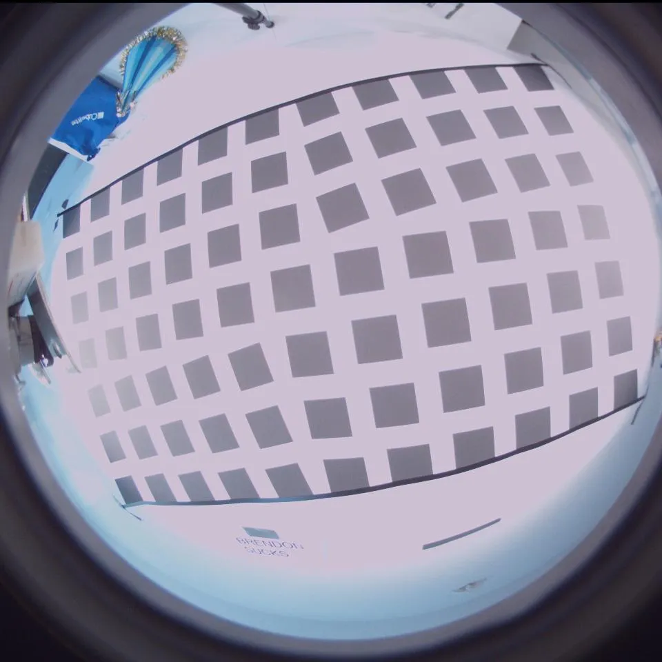
我设置的用于检索质心的流程如下： 1. 进行Canny边缘检测 2. 关注一个区域的兴趣，以最小化误报。该区域基本上是没有任何覆盖其中一侧的黑色胶带的正方形。 3. 找到所有不同的封闭轮廓 4. 对于每个不同的封闭轮廓... a. 进行Harris角点检测 b. 确定结果是否具有4个角点 c. 如果是，则此轮廓属于一个正方形，并找到该形状的质心 d. 如果不是，则跳过此形状 5. 将步骤#4中检测到的所有质心放置在矩阵中以供进一步检查。

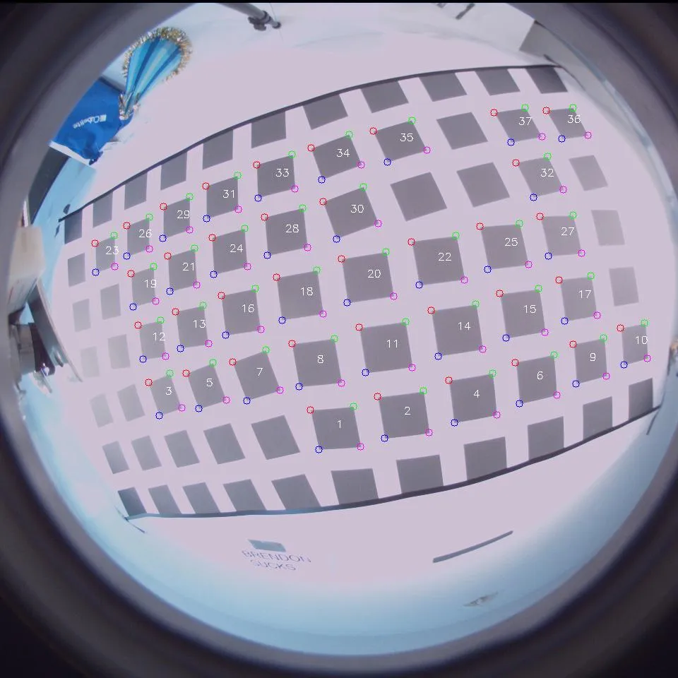
这是一个与上面图像相关的示例结果。每个检测到的正方形都有四个点，根据其相对于正方形本身的位置进行颜色编码。对于我检测到的每个质心，我会在图像中心点写下一个ID。

使用上述图像，有37个检测到的正方形。

问题设置

假设我有一些存储在N x 3矩阵中的图像像素点。前两列是x（水平）和y（垂直）坐标，在图像坐标空间中，y坐标是反转的，这意味着正的y向下移动。第三列是与该点相关联的ID。

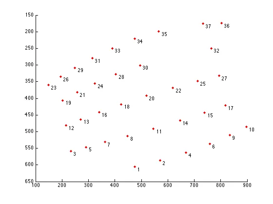
这是一些用MATLAB编写的代码，它将这些点绘制到2D网格上，并使用矩阵的第三列标记每个点。如果您阅读了上面的背景，这些是由我上面概述的算法检测到的点。

data = [ 475.  ,  605.75,    1.;
       571.  ,  586.5 ,    2.;
       233.  ,  558.5 ,    3.;
       669.5 ,  562.75,    4.;
       291.25,  546.25,    5.;
       759.  ,  536.25,    6.;
       362.5 ,  531.5 ,    7.;
       448.  ,  513.5 ,    8.;
       834.5 ,  510.  ,    9.;
       897.25,  486.  ,   10.;
       545.5 ,  491.25,   11.;
       214.5 ,  481.25,   12.;
       271.25,  463.  ,   13.;
       646.5 ,  466.75,   14.;
       739.  ,  442.75,   15.;
       340.5 ,  441.5 ,   16.;
       817.75,  421.5 ,   17.;
       423.75,  417.75,   18.;
       202.5 ,  406.  ,   19.;
       519.25,  392.25,   20.;
       257.5 ,  382.  ,   21.;
       619.25,  368.5 ,   22.;
       148.  ,  359.75,   23.;
       324.5 ,  356.  ,   24.;
       713.  ,  347.75,   25.;
       195.  ,  335.  ,   26.;
       793.5 ,  332.5 ,   27.;
       403.75,  328.  ,   28.;
       249.25,  308.  ,   29.;
       495.5 ,  300.75,   30.;
       314.  ,  279.  ,   31.;
       764.25,  249.5 ,   32.;
       389.5 ,  249.5 ,   33.;
       475.  ,  221.5 ,   34.;
       565.75,  199.  ,   35.;
       802.75,  173.75,   36.;
       733.  ,  176.25,   37.];

figure; hold on;
axis ij;
scatter(data(:,1), data(:,2),40, 'r.');
text(data(:,1)+10, data(:,2)+10, num2str(data(:,3)));

同样地，在Python中，使用numpy和matplotlib，我们有：

import numpy as np
import matplotlib.pyplot as plt

data = np.array([[ 475.  ,  605.75,    1.  ],
   [ 571.  ,  586.5 ,    2.  ],
   [ 233.  ,  558.5 ,    3.  ],
   [ 669.5 ,  562.75,    4.  ],
   [ 291.25,  546.25,    5.  ],
   [ 759.  ,  536.25,    6.  ],
   [ 362.5 ,  531.5 ,    7.  ],
   [ 448.  ,  513.5 ,    8.  ],
   [ 834.5 ,  510.  ,    9.  ],
   [ 897.25,  486.  ,   10.  ],
   [ 545.5 ,  491.25,   11.  ],
   [ 214.5 ,  481.25,   12.  ],
   [ 271.25,  463.  ,   13.  ],
   [ 646.5 ,  466.75,   14.  ],
   [ 739.  ,  442.75,   15.  ],
   [ 340.5 ,  441.5 ,   16.  ],
   [ 817.75,  421.5 ,   17.  ],
   [ 423.75,  417.75,   18.  ],
   [ 202.5 ,  406.  ,   19.  ],
   [ 519.25,  392.25,   20.  ],
   [ 257.5 ,  382.  ,   21.  ],
   [ 619.25,  368.5 ,   22.  ],
   [ 148.  ,  359.75,   23.  ],
   [ 324.5 ,  356.  ,   24.  ],
   [ 713.  ,  347.75,   25.  ],
   [ 195.  ,  335.  ,   26.  ],
   [ 793.5 ,  332.5 ,   27.  ],
   [ 403.75,  328.  ,   28.  ],
   [ 249.25,  308.  ,   29.  ],
   [ 495.5 ,  300.75,   30.  ],
   [ 314.  ,  279.  ,   31.  ],
   [ 764.25,  249.5 ,   32.  ],
   [ 389.5 ,  249.5 ,   33.  ],
   [ 475.  ,  221.5 ,   34.  ],
   [ 565.75,  199.  ,   35.  ],
   [ 802.75,  173.75,   36.  ],
   [ 733.  ,  176.25,   37.  ]])

plt.figure()
plt.gca().invert_yaxis()

plt.plot(data[:,0], data[:,1], 'r.', markersize=14)

for idx in np.arange(data.shape[0]):
    plt.text(data[idx,0]+10, data[idx,1]+10, str(int(data[idx,2])), size='large')

plt.show()

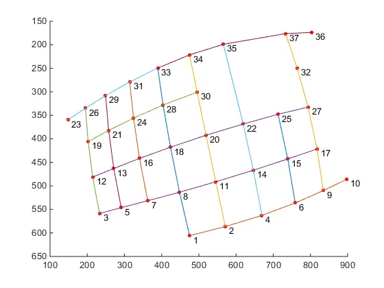
我们得到：

---

回到问题

如您所见，这些点更多或少按照网格模式排列，并且我们可以在这些点之间形成线。具体来说，您可以看到可以水平和垂直地形成线。

例如，如果您参考我问题背景中的图像，我们可以看到有5组点可以以水平方式分组。例如，点23、26、29、31、33、34、35、37和36形成一组。点19、21、24、28、30和32形成另一组，依此类推。同样，在垂直意义上，我们可以看到点26、19、12和3形成一组，点29、21、13和5形成另一组，依此类推。

---

需要问的问题

我的问题是：有什么方法可以成功地将点在水平和垂直方向上分别分组，而不管点的方向如何？

条件

1. 每条线上必须至少有三个点。如果少于三个点，则不符合要求。因此，点36和10不符合纵向线的条件，同样孤立的点23也不应该被视为一条竖向线，但它是第一个水平分组的一部分。

2. 上面的标定图案可以处于任何方向。然而，对我处理的东西来说，你能得到的最糟糕的方向是在背景部分所看到的。

---

预期输出

输出将是一对列表，其中第一个列表具有元素，每个元素都为形成水平线的点ID序列。同样，第二个列表具有元素，每个元素都为形成垂直线的点ID序列。

因此，水平序列的预期输出将类似于以下内容：

MATLAB

horiz_list = {[23, 26, 29, 31, 33, 34, 35, 37, 36], [19, 21, 24, 28, 30, 32], ...};
vert_list = {[26, 19, 12, 3], [29, 21, 13, 5], ....};

Python

horiz_list = [[23, 26, 29, 31, 33, 34, 35, 37, 36], [19, 21, 24, 28, 30, 32], ....]
vert_list = [[26, 19, 12, 3], [29, 21, 13, 5], ...]

我所尝试的

在算法上，我尝试撤销这些点所经历的旋转。我执行了主成分分析，并尝试投影基于计算的正交基向量的点，以便点大致位于一个直角坐标系网格上。

一旦我有了这个，就只需要进行一些扫描线处理，在此过程中，您可以根据水平或垂直坐标的差异对点进行分组。您可以按照x或y值对坐标进行排序，然后检查这些排序后的坐标，并寻找大的变化。一旦遇到这种变化，那么就可以将变化之间的点合并在一起形成线条。针对每个维度执行此操作将为您提供水平或垂直分组。

关于PCA，在MATLAB和Python中，我做了以下工作：

MATLAB

%# Step #1 - Get just the data - no IDs
data_raw = data(:,1:2);

%# Decentralize mean
data_nomean = bsxfun(@minus, data_raw, mean(data_raw,1));

%# Step #2 - Determine covariance matrix
%# This already decentralizes the mean
cov_data = cov(data_raw);

%# Step #3 - Determine right singular vectors
[~,~,V] = svd(cov_data);

%# Step #4 - Transform data with respect to basis
F = V.'*data_nomean.';

%# Visualize both the original data points and transformed data
figure;
plot(F(1,:), F(2,:), 'b.', 'MarkerSize', 14);
axis ij;
hold on;
plot(data(:,1), data(:,2), 'r.', 'MarkerSize', 14);

Python

import numpy as np
import numpy.linalg as la

# Step #1 and Step #2 - Decentralize mean
centroids_raw = data[:,:2]
mean_data = np.mean(centroids_raw, axis=0)

# Transpose for covariance calculation
data_nomean = (centroids_raw - mean_data).T

# Step #3 - Determine covariance matrix
# Doesn't matter if you do this on the decentralized result
# or the normal result - cov subtracts the mean off anyway
cov_data = np.cov(data_nomean)

# Step #4 - Determine right singular vectors via SVD
# Note - This is already V^T, so there's no need to transpose
_,_,V = la.svd(cov_data)

# Step #5 - Transform data with respect to basis
data_transform = np.dot(V, data_nomean).T

plt.figure()
plt.gca().invert_yaxis()

plt.plot(data[:,0], data[:,1], 'b.', markersize=14)
plt.plot(data_transform[:,0], data_transform[:,1], 'r.', markersize=14)

plt.show()

---

上述代码不仅重新投影了数据，还在单个图中同时绘制了原始点和投影点。但是，当我尝试重新投影我的数据时，得到的绘图如下：

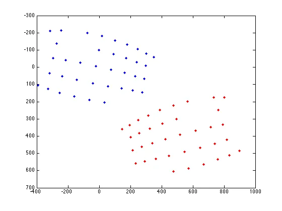
红色点是原始图像坐标，蓝色点是重新投影到基向量上的点，以尝试消除旋转。但它仍然没有完全完成任务。与这些点相关仍存在一些方向性，如果我尝试使用扫描线算法，水平跟踪下面的线或垂直跟踪侧面的线时，点会被错误地分组，这是不正确的。

---

也许我在过度思考这个问题，但是如果您有任何见解，将不胜感激。如果答案确实非常好，我会倾向于提供高额赏金，因为我已经卡在这个问题上很长时间了。

希望我的问题没有太啰嗦。如果您不知道如何解决这个问题，那么无论如何感谢您花费的时间阅读我的问题。

期待您可能拥有的任何见解。非常感谢！

- rayryeng

---

我不确定，但也许你可以通过计算凸包并先处理其边界来实现某种程度的简化... - Leandro Caniglia

@knedlsepp 感谢阅读！是的，方块也被旋转了。我没有提到这一点，因为我认为这不重要，但有些是为了通过镜头获得其他参数而旋转的。 - rayryeng

我怀疑这与bublcam有关。;-)我知道一次仿射映射在这里是不够的（而且我刚意识到应该说 projective），但我的意思是使用任意优化算法，在其中步骤你使用你试图找到和最小化误差最小的投影拟合参数变形长方形网格使用一些RANSAC方法的参数变形点和质心。 （我想您也可以将记录的点反向映射到矩形网格上，并对其进行投影适合。） - knedlsepp

@Benoit_11 - 嗯！谢谢！我总是忘记scatter :) 我会记住的，谢谢你的阅读！ - rayryeng

出于好奇，看着最顶部的图片，有没有什么原因是“Brendon sucks”？ :-) - kkuilla

Answer 1

注意1：它有若干设置 -> 对于其他图片可能需要更改以获得所需的结果 参见％设置 - 尝试调整这些值

注意2：它无法找到您想要的所有行 -> 但这是一个起点....

要调用此函数，请在命令提示符中调用此函数：

>> [h, v] = testLines;

我们得到：

>> celldisp(h)

h{1} =
     1     2     4     6     9    10
h{2} =
     3     5     7     8    11    14    15    17
h{3} =
     1     2     4     6     9    10
h{4} =
     3     5     7     8    11    14    15    17
h{5} =
     1     2     4     6     9    10
h{6} =
     3     5     7     8    11    14    15    17
h{7} =
     3     5     7     8    11    14    15    17
h{8} =
     1     2     4     6     9    10
h{9} =
     1     2     4     6     9    10
h{10} =
    12    13    16    18    20    22    25    27
h{11} =
    13    16    18    20    22    25    27
h{12} =
     3     5     7     8    11    14    15    17
h{13} =
     3     5     7     8    11    14    15
h{14} =
    12    13    16    18    20    22    25    27
h{15} =
     3     5     7     8    11    14    15    17
h{16} =
    12    13    16    18    20    22    25    27
h{17} =
    19    21    24    28    30
h{18} =
    21    24    28    30
h{19} =
    12    13    16    18    20    22    25    27
h{20} =
    19    21    24    28    30
h{21} =
    12    13    16    18    20    22    24    25
h{22} =
    12    13    16    18    20    22    24    25    27
h{23} =
    23    26    29    31    33    34    35
h{24} =
    23    26    29    31    33    34    35    37
h{25} =
    23    26    29    31    33    34    35    36    37
h{26} =
    33    34    35    37    36
h{27} =
    31    33    34    35    37

>> celldisp(v)
v{1} =
    33    28    18     8     1
v{2} =
    34    30    20    11     2
v{3} =
    26    19    12     3
v{4} =
    35    22    14     4
v{5} =
    29    21    13     5
v{6} =
    25    15     6
v{7} =
    31    24    16     7
v{8} =
    37    32    27    17     9

还会生成一幅图，通过每组正确的点绘制线条：

function [horiz_list, vert_list] = testLines

global counter;
global colours; 
close all;

data = [ 475.  ,  605.75,    1.;
       571.  ,  586.5 ,    2.;
       233.  ,  558.5 ,    3.;
       669.5 ,  562.75,    4.;
       291.25,  546.25,    5.;
       759.  ,  536.25,    6.;
       362.5 ,  531.5 ,    7.;
       448.  ,  513.5 ,    8.;
       834.5 ,  510.  ,    9.;
       897.25,  486.  ,   10.;
       545.5 ,  491.25,   11.;
       214.5 ,  481.25,   12.;
       271.25,  463.  ,   13.;
       646.5 ,  466.75,   14.;
       739.  ,  442.75,   15.;
       340.5 ,  441.5 ,   16.;
       817.75,  421.5 ,   17.;
       423.75,  417.75,   18.;
       202.5 ,  406.  ,   19.;
       519.25,  392.25,   20.;
       257.5 ,  382.  ,   21.;
       619.25,  368.5 ,   22.;
       148.  ,  359.75,   23.;
       324.5 ,  356.  ,   24.;
       713.  ,  347.75,   25.;
       195.  ,  335.  ,   26.;
       793.5 ,  332.5 ,   27.;
       403.75,  328.  ,   28.;
       249.25,  308.  ,   29.;
       495.5 ,  300.75,   30.;
       314.  ,  279.  ,   31.;
       764.25,  249.5 ,   32.;
       389.5 ,  249.5 ,   33.;
       475.  ,  221.5 ,   34.;
       565.75,  199.  ,   35.;
       802.75,  173.75,   36.;
       733.  ,  176.25,   37.];

figure; hold on;
axis ij;

% Change due to Benoit_11
scatter(data(:,1), data(:,2),40, 'r.'); text(data(:,1)+10, data(:,2)+10, num2str(data(:,3)));
text(data(:,1)+10, data(:,2)+10, num2str(data(:,3)));

% Process your data as above then run the function below(note it has sub functions)
counter = 0;
colours = 'bgrcmy';
[horiz_list, vert_list] = findClosestPoints ( data(:,1), data(:,2) );


function [horiz_list, vert_list] = findClosestPoints ( x, y )
  % calc length of points
  nX = length(x);
  % set up place holder flags
  modelledH = false(nX,1);
  modelledV = false(nX,1);
  horiz_list = {};
  vert_list = {};

  % loop for all points
  for p=1:nX
    % have we already modelled a horizontal line through these?
    % second last param - true - horizontal, false - vertical
    if modelledH(p)==false
      [modelledH, index] = ModelPoints ( p, x, y, modelledH, true, true );
      horiz_list = [horiz_list index];
    else
      [~, index] = ModelPoints ( p, x, y, modelledH, true, false );
      horiz_list = [horiz_list index];
    end

    % make a temp copy of the x and y and remove any of the points modelled 
    %  from the horizontal -> this  is to avoid them being found in the 
    %  second call.
    tempX = x;
    tempY = y;
    tempX(index) = NaN;
    tempY(index) = NaN;
    tempX(p) = x(p);
    tempY(p) = y(p);
    % Have we found a vertial line?
    if modelledV(p)==false
      [modelledV, index] = ModelPoints ( p, tempX, tempY, modelledV, false, true );
      vert_list = [vert_list index];
    end
  end
end
function [modelled, index] = ModelPoints ( p, x, y, modelled, method, fullRun )
  % p - row in your original data matrix
  % x - data(:,1)
  % y - data(:,2)
  % modelled - array of flags to whether rows have been modelled
  % method   - horizontal or vertical (used to calc graadients)
  % fullRun  - full calc or just to get indexes 
  %            this could be made better by storing the indexes of each horizontal in the method above

  % Settings - play around with these values 
  gradDelta = 0.2;  % find points where gradient is less than this value
  gradLimit = 0.45; % if mean gradient of line is above this ignore
  numberOfPointsToCheck = 7; % number of points to check when look along the line
                        % to find other points (this reduces chance of it
                        % finding other points far away
                        %  I optimised this for your example to be 7
                        %  Try varying it and you will see how it effect the result.

  % Find the index of points which are inline.
  [index, grad] = CalcIndex ( x, y, p, gradDelta, method );
  % check gradient of line
  if abs(mean(grad))>gradLimit
    index = [];
    return
  end
  % add point of interest to index
  index = [p index];

  % loop through all points found above to find any other points which are in
  %  line with these points (this allows for slight curvature
  combineIndex = [];
  for ii=2:length(index)
    % Find inedex of the points found above (find points on curve)
    [index2] = CalcIndex ( x, y, index(ii), gradDelta, method, numberOfPointsToCheck, grad(ii-1) );

    % Check that the point on this line are on the original (i.e. inline -> not at large angle
    if any(ismember(index,index2))
      % store points found
      combineIndex = unique([index2 combineIndex]);
    end
  end

  % copy to index
  index = combineIndex;
  if fullRun
    %  do some plotting
    %  TODO: here you would need to calculate your arrays to output.
    xx = x(index);
    [sX,sOrder] = sort(xx);
    % Check its found at least 3 points
    if length ( index(sOrder) ) > 2
      % flag the modelled on the points found
      modelled(index(sOrder)) = true;
      % plot the data
      plot ( x(index(sOrder)), y(index(sOrder)), colours(mod(counter,numel(colours)) + 1));
      counter = counter + 1;
    end
    index = index(sOrder);
  end
end  
function [index, gradCheck] = CalcIndex ( x, y, p, gradLimit, method, nPoints2Consider, refGrad )
  % x - data(:,1)
  % y - data(:,2)
  % p - point of interest
  % method (x/y) or (y\x)
  % nPoints2Consider - only look at N points (options)
  % refgrad          - rather than looking for gradient of closest point -> use this
  %                  - reference gradient to find similar points (finds points on curve)
  nX = length(x);
  % calculate gradient
  for g=1:nX
    if method
      grad(g) = (x(g)-x(p))\(y(g)-y(p));
    else
      grad(g) = (y(g)-y(p))\(x(g)-x(p));
    end
  end
  % find distance to all other points
  delta = sqrt ( (x-x(p)).^2 + (y-y(p)).^2 );
  % set its self = NaN
  delta(delta==min(delta)) = NaN;
  % find the closest points
  [m,order] = sort(delta);

  if nargin == 7
    % for finding along curve
    % set any far away points to be NaN
    grad(order(nPoints2Consider+1:end)) = NaN;
    % find the closest points to the reference gradient within the allowable limit
    index = find(abs(grad-refGrad)<gradLimit==1);
    % store output
    gradCheck = grad(index);
  else
    % find the points which are closes to the gradient of the closest point
    index = find(abs(grad-grad(order(1)))<gradLimit==1);
    % store gradients to output
    gradCheck = grad(index);
  end
end
end

- matlabgui

---

正要发表类似的内容！顺便说一下：您可以使用“knnsearch”完成大部分手动工作 https://gist.github.com/knedlsepp/5a62e16d22d01ab38f56 然后我建议找到连接点处角度较小的相邻边。这样就可以删除错误的对角线边缘。 - knedlsepp

@rayryeng 祝你好运! :) 很高兴能够提供帮助! 我认为这是一个有趣的问题，我有一些空闲时间可以在咨询和我的 GUI 工具箱之外工作。 - matlabgui

@matlabgui - 悬赏已发放！非常感谢您的耐心等待。保重！ - rayryeng

@JuliaKoncha 嗯，这是很久以前的事情了！如果我没记错的话，我写的算法是在Matlab中没有任何工具箱的情况下完成的，所以我想你应该能够用其他任何语言来实现它。 - matlabgui

@JuliaKoncha 没问题。我想我可能会有时间在这个周末完成它。转换应该非常简单。完成后，我可能会将其放在GitHub上，您可以在必要时使用和修改。同时祝你好运！ - rayryeng

Answer 2

我正在使用输入的裁剪版本的图像。在这里，我只讨论可以将网格方向视为近似水平/垂直的情况。这可能不能完全涵盖您的范围，但我认为它可能会给您一些指示。

将图像二值化，使扭曲的正方形填充。这里我使用简单的Otsu阈值处理。然后对此二进制图像进行距离变换。

在距离变换图像中，我们看到正方形之间的间隙作为峰值。

要获得水平方向的线条，请获取距离图像的每个列的局部极大值，然后查找连接的组件。

要获得垂直方向的线条，请获取距离图像的每个行的局部极大值，然后查找连接的组件。

下面的图像显示了找到的水平线和垂直线，其中角点为圆圈。

对于相当长的连接组件，可以拟合曲线（线或多项式），然后分类角点，例如基于到曲线的距离，在曲线的哪一侧是点等。

我在Matlab中完成了这项工作。我没有尝试拟合曲线和分类部分。

clear all;
close all;

im = imread('0RqUd-1.jpg');
gr = rgb2gray(im);
% any preprocessing to get a binary image that fills the distorted squares
bw = ~im2bw(gr, graythresh(gr));

di = bwdist(bw);                % distance transform
di2 = imdilate(di, ones(3));    % propagate max

corners = corner(gr);           % simple corners

% find regional max for each column of dist image
regmxh = zeros(size(di2));
for c = 1:size(di2, 2)
    regmxh(:, c) = imregionalmax(di2(:, c));
end
% label connected components
ccomph = bwlabel(regmxh, 8);

% find regional max for each row of dist image
regmxv = zeros(size(di2));
for r = 1:size(di2, 1)
    regmxv(r, :) = imregionalmax(di2(r, :));
end
% label connected components
ccompv = bwlabel(regmxv, 8);

figure, imshow(gr, [])
hold on
plot(corners(:, 1), corners(:, 2), 'ro')
figure, imshow(di, [])
figure, imshow(label2rgb(ccomph), [])
hold on
plot(corners(:, 1), corners(:, 2), 'ro')
figure, imshow(label2rgb(ccompv), [])
hold on
plot(corners(:, 1), corners(:, 2), 'ro')

为了获得任意定向网格的这些线条，您可以将距离图像视为图形并找到最佳路径。有一个很好的基于图形的方法，请参见此处。

- dhanushka

---

感谢您的方法。+1。然而，我将选择matlabgui的方法，因为它不需要图像处理工具箱中的任何内容。此外，最终算法将在Python中执行，因此他的解决方案更具可移植性。尽管如此，还是非常感谢您的努力！ - rayryeng

Answer 3

虽然我无法建议比您已经尝试过的更好的方法来分组任何给定的质心点，但我希望以下想法可能会帮助您：

由于您非常关注图像的内容（包含一个正方形场），所以我想知道您是否实际上需要从您的“问题设置”中给出的数据中分组质心点，还是您可以使用在“问题背景”中描述的数据。由于您已经确定了每个检测到的正方形的角落以及它们在该给定正方形中的位置，因此对于通过比较角坐标来确定给定正方形的邻居，这似乎对我来说非常准确。

因此，为了找到任何正方形的右邻居的候选者，我建议您将该正方形的右上角和右下角与任何其他正方形（或任何一定距离内的任何正方形）的左上角和左下角进行比较。只允许小的垂直差异和稍大的水平差异，如果两个相应的角点都足够接近，您可以将两个正方形“匹配”。

通过使用允许的垂直/水平角差异的上限，您甚至可能能够仅将最佳匹配的正方形分配为邻居。

问题可能是您没有检测到所有正方形，因此正方形30和32之间的空间相当大。由于您说您需要每行“至少”3个正方形，因此对于您来说，在该水平线上简单地忽略正方形32可能是可行的选择。如果这对您不是一个选项，您可以尝试尽可能匹配正方形，然后使用先前计算的数据将“缺失”的正方形分配到网格中的某个点：

在关于正方形32的示例中，您将会检测到它有27和37两个上下邻居。此外，您应该能够确定正方形27位于第1行，而正方形37位于第3行，因此您可以将正方形32分配给它们之间最佳匹配的行，显然在这种情况下是第2行。

这种一般方法基本上是您已经尝试过的方法，但应该更准确，因为现在您正在比较两条线的方向和距离，而不仅仅是比较网格中两个点的位置。

另外，关于您以前的尝试-您能否使用黑色角线来稍微校正图像的初始旋转？这可能会使进一步的扭曲算法（如您在评论中与knedlsepp讨论的算法）更加准确。（编辑：我刚刚读了Parag的评论-通过线的角度比较点当然基本上与预先旋转图像相同）

- H W

---

1. 我不仅需要考虑质心。我当然可以使用图像中可用的任何数据，所以你肯定可以利用那些信息。
2. 我当然可以避免使用32像素的正方形来表示水平线。同一行上的其他质心分布得足够好，可以被视为共线。
3. 谢谢你的关注 :) 我很可能会将你的想法与matlabgui提供给我的内容结合起来使用。保重！

- rayryeng