提高图像处理精度以计算真菌孢子数量

Question

我正在尝试使用Python从显微镜样本中计算一种疾病的孢子数量，但迄今为止没有太大成功。

由于孢子的颜色与背景相似，并且许多孢子非常接近。

根据样本的显微摄影结果进行操作。

图像处理代码：

import numpy as np
import argparse
import imutils
import cv2

ap = argparse.ArgumentParser()
ap.add_argument("-i", "--image", required=True,
                help="path to the input image")
ap.add_argument("-o", "--output", required=True,
                help="path to the output image")
args = vars(ap.parse_args())

counter = {}

image_orig = cv2.imread(args["image"])
height_orig, width_orig = image_orig.shape[:2]

image_contours = image_orig.copy()

colors = ['Yellow']
for color in colors:

    image_to_process = image_orig.copy()

    counter[color] = 0

    if color == 'Yellow':
        lower = np.array([70, 150, 140])  #rgb(151, 143, 80)
        upper = np.array([110, 240, 210])  #rgb(212, 216, 106)

    image_mask = cv2.inRange(image_to_process, lower, upper)

    image_res = cv2.bitwise_and(
        image_to_process, image_to_process, mask=image_mask)

    image_gray = cv2.cvtColor(image_res, cv2.COLOR_BGR2GRAY)
    image_gray = cv2.GaussianBlur(image_gray, (5, 5), 50)

    image_edged = cv2.Canny(image_gray, 100, 200)
    image_edged = cv2.dilate(image_edged, None, iterations=1)
    image_edged = cv2.erode(image_edged, None, iterations=1)

    cnts = cv2.findContours(
        image_edged.copy(), cv2.RETR_EXTERNAL, cv2.CHAIN_APPROX_SIMPLE)
    cnts = cnts[0] if imutils.is_cv2() else cnts[1]

    for c in cnts:

        if cv2.contourArea(c) < 1100:
            continue

        hull = cv2.convexHull(c)
        if color == 'Yellow':

            cv2.drawContours(image_contours, [hull], 0, (0, 0, 255), 1)

        counter[color] += 1      

print("{} esporos {}".format(counter[color], color))

cv2.imwrite(args["output"], image_contours)

该算法计数11孢子。

但是图像中包含27个孢子

图像处理结果显示孢子被分组

如何使这更准确？

- Georg Augusto

---

计算机视觉中有很多关于分离接近或相邻斑点的研究，你可以在学术搜索引擎Scholar或普通Google上查找相关论文。例如，“computer vision separating close by blobs”可以找到这篇文章：Detection and Segmentation of Multiple Touching Product Inspection Items。但一般来说，你可能需要进行多次腐蚀操作才能达到预期效果。 - Roope

“Watershed” 算法可能有效。 - kkuilla

虽然不是完全一样的问题，但此处提供的另一个问题将帮助您找到更好的方法来分离您的对象：https://dev59.com/dlvUa4cB1Zd3GeqPr0jp — 基于分水岭的方法是解决此问题的常见方法。 - Cris Luengo

Answer 1

首先，我们需要一些预备代码，下面将会用到它：

import numpy as np
import cv2
from matplotlib import pyplot as plt
from skimage.morphology import extrema
from skimage.morphology import watershed as skwater

def ShowImage(title,img,ctype):
  if ctype=='bgr':
    b,g,r = cv2.split(img)       # get b,g,r
    rgb_img = cv2.merge([r,g,b])     # switch it to rgb
    plt.imshow(rgb_img)
  elif ctype=='hsv':
    rgb = cv2.cvtColor(img,cv2.COLOR_HSV2RGB)
    plt.imshow(rgb)
  elif ctype=='gray':
    plt.imshow(img,cmap='gray')
  elif ctype=='rgb':
    plt.imshow(img)
  else:
    raise Exception("Unknown colour type")
  plt.title(title)
  plt.show()

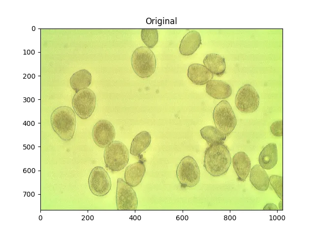
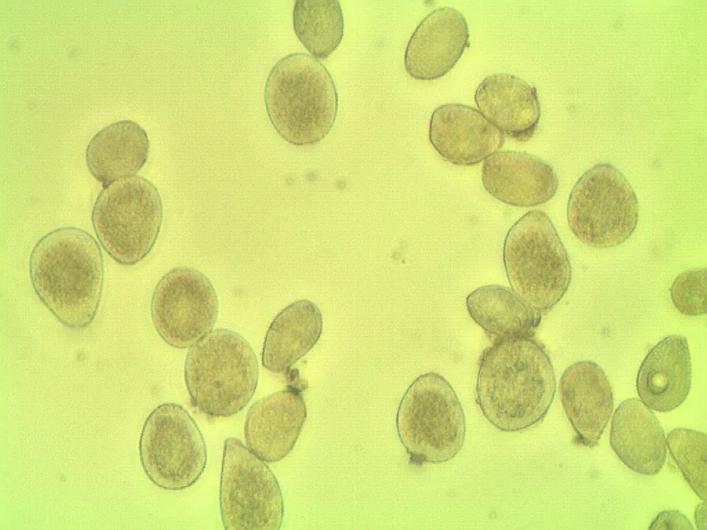
供参考，这是您的原始图像：

#Read in image
img         = cv2.imread('cells.jpg')
ShowImage('Original',img,'bgr')

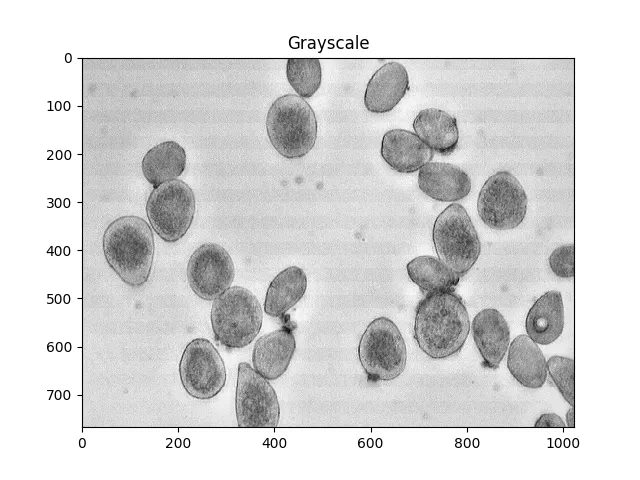
大津法是一种分割颜色的方法。该方法假设图像像素的强度可以绘制成双峰直方图，并找到该直方图的最佳分隔符。我在下面应用了这种方法。

#Convert to a single, grayscale channel
gray        = cv2.cvtColor(img,cv2.COLOR_BGR2GRAY)
#Threshold the image to binary using Otsu's method
ret, thresh = cv2.threshold(gray,0,255,cv2.THRESH_BINARY_INV+cv2.THRESH_OTSU)
ShowImage('Grayscale',gray,'gray')
ShowImage('Applying Otsu',thresh,'gray')

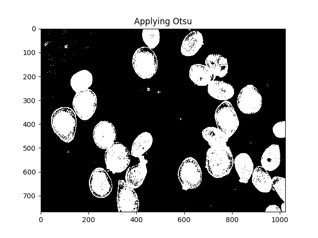
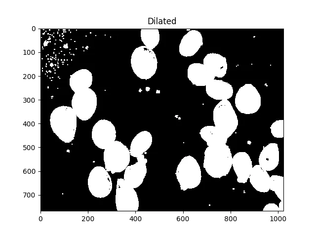
所有这些小斑点都很烦人，我们可以通过膨胀来消除它们：

#Adjust iterations until desired result is achieved
kernel  = np.ones((3,3),np.uint8)
dilated = cv2.dilate(thresh, kernel, iterations=5)
ShowImage('Dilated',dilated,'gray')

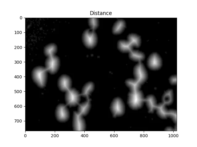
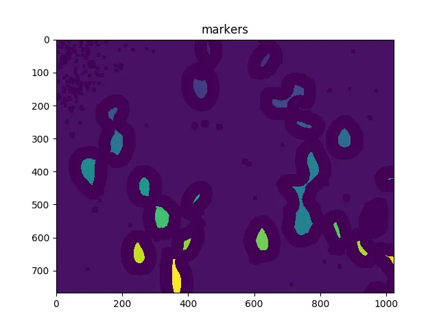
现在我们需要确定分水岭的峰值并给它们单独的标签。这样做的目的是生成一组像素，使每个单元格内都有一个像素，并且没有两个单元格的标识符像素相接触。

为了实现这一点，我们执行距离变换，然后过滤掉距离细胞中心太远的距离。

#Calculate distance transformation
dist         = cv2.distanceTransform(dilated,cv2.DIST_L2,5)
ShowImage('Distance',dist,'gray')

#Adjust this parameter until desired separation occurs
fraction_foreground = 0.6
ret, sure_fg = cv2.threshold(dist,fraction_foreground*dist.max(),255,0)
ShowImage('Surely Foreground',sure_fg,'gray')

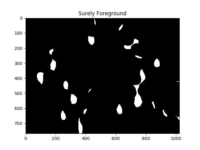
以上图像中的每个白色区域在算法看来都是一个单独的单元。

现在，我们通过减去最大值来识别未知区域，即将由分水岭算法标记的区域：

# Finding unknown region
unknown = cv2.subtract(dilated,sure_fg.astype(np.uint8))
ShowImage('Unknown',unknown,'gray')

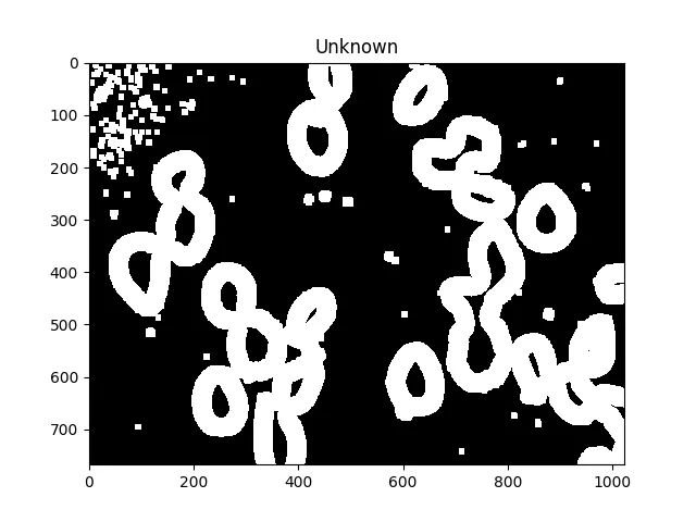
未知区域应该在每个单元格周围形成完整的甜甜圈。

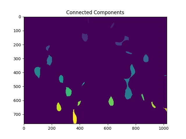
接下来，我们为距离变换产生的每个不同区域分配唯一标签，然后标记未知区域，最后执行分水岭变换：

# Marker labelling
ret, markers = cv2.connectedComponents(sure_fg.astype(np.uint8))
ShowImage('Connected Components',markers,'rgb')

# Add one to all labels so that sure background is not 0, but 1
markers = markers+1

# Now, mark the region of unknown with zero
markers[unknown==np.max(unknown)] = 0

ShowImage('markers',markers,'rgb')

dist    = cv2.distanceTransform(dilated,cv2.DIST_L2,5)
markers = skwater(-dist,markers,watershed_line=True)

ShowImage('Watershed',markers,'rgb')

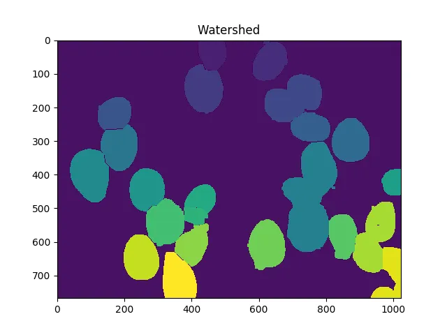
现在单元格的总数是唯一标记数量减1（忽略背景）：

len(set(markers.flatten()))-1

在这种情况下，我们得到了23。

通过调整距离阈值、膨胀程度，可能使用h-maxima（局部阈值最大值）等方法，可以使其更加准确或不准确。但要注意过度拟合；也就是说，不要假设为单个图像进行调整将在任何地方都给出最佳结果。

估计不确定性

您还可以通过算法略微改变参数来了解计数中的不确定性。这可能看起来像这样：

import numpy as np
import cv2
import itertools
from matplotlib import pyplot as plt
from skimage.morphology import extrema
from skimage.morphology import watershed as skwater

def CountCells(dilation=5, fg_frac=0.6):
  #Read in image
  img         = cv2.imread('cells.jpg')
  #Convert to a single, grayscale channel
  gray        = cv2.cvtColor(img,cv2.COLOR_BGR2GRAY)
  #Threshold the image to binary using Otsu's method
  ret, thresh = cv2.threshold(gray,0,255,cv2.THRESH_BINARY_INV+cv2.THRESH_OTSU)
  #Adjust iterations until desired result is achieved
  kernel  = np.ones((3,3),np.uint8)
  dilated = cv2.dilate(thresh, kernel, iterations=dilation)
  #Calculate distance transformation
  dist         = cv2.distanceTransform(dilated,cv2.DIST_L2,5)
  #Adjust this parameter until desired separation occurs
  fraction_foreground = fg_frac
  ret, sure_fg = cv2.threshold(dist,fraction_foreground*dist.max(),255,0)
  # Finding unknown region
  unknown = cv2.subtract(dilated,sure_fg.astype(np.uint8))
  # Marker labelling
  ret, markers = cv2.connectedComponents(sure_fg.astype(np.uint8))
  # Add one to all labels so that sure background is not 0, but 1
  markers = markers+1
  # Now, mark the region of unknown with zero
  markers[unknown==np.max(unknown)] = 0    
  markers = skwater(-dist,markers,watershed_line=True)
  return len(set(markers.flatten()))-1

#Smaller numbers are noisier, which leads to many small blobs that get
#thresholded out (undercounting); larger numbers result in possibly fewer blobs,
#which can also cause undercounting.
dilations = [4,5,6] 
#Small numbers equal less separation, so undercounting; larger numbers equal
#more separation or drop-outs. This can lead to over-counting initially, but
#rapidly to under-counting.
fracs     = [0.5, 0.6, 0.7, 0.8] 

for params in itertools.product(dilations,fracs):
  print("Dilation={0}, FG frac={1}, Count={2}".format(*params,CountCells(*params)))

给出结果：

Dilation=4, FG frac=0.5, Count=22
Dilation=4, FG frac=0.6, Count=23
Dilation=4, FG frac=0.7, Count=17
Dilation=4, FG frac=0.8, Count=12
Dilation=5, FG frac=0.5, Count=21
Dilation=5, FG frac=0.6, Count=23
Dilation=5, FG frac=0.7, Count=20
Dilation=5, FG frac=0.8, Count=13
Dilation=6, FG frac=0.5, Count=20
Dilation=6, FG frac=0.6, Count=23
Dilation=6, FG frac=0.7, Count=24
Dilation=6, FG frac=0.8, Count=14

取计数值的中位数是将不确定性合并为一个数字的一种方法。

请记住，StackOverflow的许可要求您给予适当的 归属。在学术工作中，可以通过引用来完成此操作。

- Richard

---

只是出于好奇，你花了多少时间在这上面？ - kkuilla

@kkuilla：可能不到30分钟。我对这组技术非常熟悉。如果想做得更好需要更多的实验和时间，但我认为这已经足够让OP开始了。 - Richard

Answer 2

这些真菌孢子大小相差不大，如果你不需要非常精确的准确度，可以通过对当前算法进行简单的更改来获得更高的准确性，而不必深入研究扩展边界和分水岭。在此场景中，孢子具有类似的大小和基本均匀的形状。因此，您可以使用轮廓的面积以及平均孢子面积来找到大约占据该区域的孢子数量。孢子无法完全填充这些任意形状，因此您需要考虑这一点。您可以通过查找背景颜色并从轮廓面积中删除背景颜色占用的区域来实现这一点。在这种情况下，您应该能够非常接近于细胞面积的真实值。

总结如下：

- 查找孢子的平均面积 - 查找背景颜色 - 查找轮廓面积 - 从轮廓中减去背景颜色像素/面积 - 近似孢子数量= ceil（轮廓面积/（孢子平均面积））

您在这里使用ceil来处理可能单独找到的小于平均值的孢子的情况，尽管您也可以放置一个特定条件来处理此问题，但是然后您必须决定是否要计算一颗孢子的分数或将其四舍五入为轮廓面积大于孢子的平均面积的整数。

但是，您可能会注意到，如果您可以确定背景颜色并且您的孢子大致相同形状和均匀颜色，则从整个图像中减去背景颜色的面积并将平均孢子大小除以剩余面积的方法在性能方面更好。这比使用膨胀快得多。

另外一件你应该考虑的事情，虽然我不认为这会解决你的团块问题，就是使用OpenCV内置的Blob检测，如果你选择面积方法，可能能够帮助你处理背景梯度所呈现的边缘情况。使用blob检测，你可以检测到blob，并将总blob面积除以平均孢子面积。你可以查看这个教程来了解如何在Python中使用它。你也可以发现使用OpenCV轮廓的简单轮廓方法对于你的用例有帮助。 简而言之：你的孢子大小和颜色大致相同，背景大致均匀，使用平均孢子面积并将孢子颜色占据的面积除以总面积，可以得到更准确的计数

附录：

如果您在寻找平均孢子面积方面遇到困难，那么如果您有关于孢子的平均“孤独”程度（明显分离程度）的任何想法，您可以使用该想法来按面积排序轮廓/斑点，然后根据“孤独”概率（n）取底部n％的孢子，并对其进行平均。只要“孤独”不太依赖于孢子大小，这应该是平均孢子大小的相当准确的测量方法。这种方法之所以有效，是因为如果假设孢子的“孤独”分布是均匀的，那么您可以将其视为自己的随机样本，如果您知道孤独百分比的平均值，那么您将很可能获得非常高的孤独孢子百分比，如果您按大小排序的孢子中取%n（或略微缩小n以降低意外捕获大孢子的概率）。如果您知道缩放因子，理论上只需要执行一次此操作。

- Krupip